Several Key PerformanceAnalytics Functions From R Now In Python (special thanks to Vijay Vaidyanathan)

So, thanks to my former boss, and head of direct indexing at BNY Mellon, Vijay Vaidyanathan, and his Coursera course, along with the usual assistance from chatGPT (I officially see it as a pseudo programming language), I have some more software for the Python community now released to my github. As wordpress now makes it very difficult to paste formatted code, I’ll be linking more often to github files.

In today’s post, the code in question is a python file containing quite a few functions from R’s PerformanceAnalytics library outside of Return.portfolio (or Return_portfolio, as it may be in Python, because the . operator is reserved in Python…ugh).

So, here is the “library” of new functions, for now called edhec_perfa.py, as a nod to Vijay Vaidyanathan’s Coursera course(s).

Here’s the link to the latest github file.

Now, while a lot of the functions should be pretty straightforward (annualized return, VaR, CVaR, tracking error/annualized tracking error, etc.), two functions that I think are particularly interesting that I ported over from R with the help of chatGPT (seriously, when prompted correctly, an LLM is quite helpful in translating from one programming language to another, provided the programmer has enough background in both languages to do various debugging) are charts_PerformanceSummary, which does exactly what you might think it does from seeing me use the R function here on the blog, and table_Drawdowns, which gives the highest N drawdowns by depth.

Here’s a quick little Python demo (once you import my file from the github):

import yfinance as yf
import pandas as pd
import numpy as np

symbol = "SPY"
start_date = "1990-01-01"
end_date = pd.Timestamp.today().strftime("%Y-%m-%d")
df_list = []

data = pd.DataFrame(yf.download(symbol, start=start_date, end=end_date))
data = data["Adj Close"]
data.name = symbol
data = pd.DataFrame(data)

returns = Return_calculate(data)

charts_PerformanceSummary(returns)
table_Drawdowns(returns)

This results in the following:

And the following table:

The NaT in the “To” column means that the drawdown is current, as does the NaN in the Recovery–they’re basically Python’s equivalent of NAs, though NaT means an NA on *time*, while an NaN means an NA on a numerical value. So that’s interesting in that Python gives you a little more information regarding your column data types, which is kind of interesting.

Another function included in this library, as a utility function is the infer_trading_periods function. Simply, plug in a time series, and it will tell you the periodicity of the data. Pandas was supposed to have a function that did this, but due to differences in frequency of daily data caused by weekends and holidays, this actually doesn’t work on financial data, so I worked with chatGPT to write a new function that works more generally. R’s checkData function is also in this library (translated over to Python), but I’m not quite sure where it was intended to be used, but left it in for those that want it.

So, for those interested, just feel free to read through some of the functions, and use whichever ones you find applicable to your workflow. That said, if you *do* wind up using it, please let me know, since there’s more value I can add.

Lastly, I’m currently in the job market *and* have a volatility trading signal subscription available to offer for those interested. You can email me at ilya.kipnis@gmail.com or find me on my LinkedIn profile here.

Thanks for reading.

A Python Investigation of a New Proposed Short Vol ETF–SVIX

This post will be about analyzing SVIX–a proposed new short vol ETF that aims to offer the same short vol exposure as XIV used to–without the downside of, well, blowing up in 20 minutes due to positive feedback loops. As I’m currently enrolled in a Python bootcamp, this was one of my capstone projects on A/B testing, so, all code will be in Python (again).

So, first off, with those not familiar, there was an article about this proposed ETF published about a month ago. You can read it here. The long story short is that this ETF is created by one Stuart Barton, who also manages InvestInVol. From conversations with Stuart, I can vouch for the fact that he strikes me as very knowledgeable in the vol space, and, if I recall correctly, was one of the individuals that worked on the original VXX ETF at Barclay’s. So when it comes to creating a newer, safer vehicle for trading short-term short vol, I’d venture to think he’s about as good as any.

In any case, here’s a link to my Python notebook, ahead of time, which I will now discuss here, on this post.

So first off, we’ll start by getting the data, and in case anyone forgot what XIV did in 2018, here’s a couple of plots.

import numpy as np
import pandas as pd
import scipy.stats as stats
import matplotlib.pyplot as plt
from pandas_datareader import data
import datetime as dt
from datetime import datetime

# get XIV from a public dropbox -- XIV had a termination event Feb. 5 2018, so this is archived data.

xiv = pd.read_csv("https://dl.dropboxusercontent.com/s/jk6der1s5lxtcfy/XIVlong.TXT", parse_dates=True, index_col=0)

# get SVXY data from Yahoo finance
svxy = data.DataReader('SVXY', 'yahoo', '2016-01-01')
#yahoo_xiv = data.DataReader('XIV', 'yahoo', '1990-01-01')

# yahoo no longer carries XIV because the instrument blew up, need to find it from historical sources
xiv_returns = xiv['Close'].pct_change()
svxy_returns = svxy['Close'].pct_change()

xiv['Close'].plot(figsize=(20,10))
plt.show()
xiv['2016':'2018']['Close'].plot(figsize=(20,10))

Yes, for those new to the blog, that event actually happened, and in the span of 20 minutes (my trading system got to the sideline about a week before, and even had I been in–which I wasn’t–I would have been in ZIV), during which time XIV blew up in after-hours trading. Immediately following, SVXY (which survived), deleveraged to a 50% exposure.

In any case, here’s the code to get SVIX data from my dropbox, essentially to the end of 2019, after I manually did some work on it because the CBOE has it in a messy format, and then to combine it with the combined XIV + SVXY returns data. (For the record, the SVIX hypothetical performance can be found here on the CBOE website)

# get formatted SVIX data from my dropbox (CBOE has it in a mess)

svix = pd.read_csv("https://www.dropbox.com/s/u8qiz7rh3rl7klw/SHORTVOL_Data.csv?raw=1", header = 0, parse_dates = True, index_col = 0)
svix.columns = ["Open", "High", "Low", "Close"]
svix_rets = svix['Close'].pct_change()

# put data set together

xiv_svxy = pd.concat([xiv_returns[:'2018-02-07'],svxy_returns['2018-02-08':]], axis = 0)
xiv_svxy_svix = pd.concat([xiv_svxy, svix_rets], axis = 1).dropna()
xiv_svxy_svix.tail()

final_data = xiv_svxy_svix
final_data.columns = ["XIV_SVXY", "SVIX"]

One thing that can be done right off the bat (which is a formality) is check if the distributions of XIV+SVXY or SVIX are normal in nature.

print(stats.describe(final_data['XIV_SVXY']))
print(stats.describe(final_data['SVIX']))
print(stats.describe(np.random.normal(size=10000)))

Which gives the following output:

DescribeResult(nobs=3527, minmax=(-0.9257575757575758, 0.1635036496350366), mean=0.0011627123490346562, variance=0.0015918321320673623, skewness=-4.325358554250933, kurtosis=85.06927230848028)
DescribeResult(nobs=3527, minmax=(-0.3011955533480766, 0.16095949898733686), mean=0.0015948970447533636, variance=0.0015014216189676208, skewness=-1.0811171524703087, kurtosis=4.453114992142524)
DescribeResult(nobs=10000, minmax=(-4.024990382591559, 4.017237262611489), mean=-0.012317646021121993, variance=0.9959681097965573, skewness=0.00367629631713188, kurtosis=0.0702696931810931)

Essentially, both of them are very non-normal (obviously), so any sort of statistical comparison using t-tests isn’t really valid. That basically leaves the Kruskal-Wallis test and Wilcoxon signed rank test to see if two data sets are different. From a conceptual level, the idea is fairly straightforward: the Kruskal-Wallis test is analogous to a two-sample independent t-test to see if one group differs from another, while the Wilcoxon signed rank test is analogous to a t-test of differences, except both use ranks of the observations rather than the actual values themselves.

Here’s the code for that:

stats.kruskal(final_data['SVIX'], final_data['XIV_SVXY'])
stats.wilcoxon(final_data['SVIX'], final_data['XIV_SVXY'])

With the output:

KruskalResult(statistic=0.8613306385456933, pvalue=0.3533665896055551)
WilcoxonResult(statistic=2947901.0, pvalue=0.0070668195307847575)

Essentially, when seen as two completely independent instruments, there isn’t enough statistical evidence to reject the idea that SVIX has no difference in terms of the ranks of its returns compared to XIV + SVXY, which would make a lot of sense, considering that for both, Feb. 5, 2018 was their worst day, and there wasn’t much of a difference between the two instruments prior to Feb. 5. In contrast, when considering the two instruments from the perspective of SVIX becoming the trading vehicle for what XIV used to be, and then comparing the differences against a 50% leveraged SVXY, then SVIX is the better instrument with differences that are statistically significant at the 1% level.

Basically, SVIX accomplishes its purpose of being an improved take on XIV/SVXY, because it was designed to be just that, with statistical evidence of exactly this.

One other interesting question to ask is when exactly did the differences in the Wilcoxon signed rank test start appearing? After all, SVIX is designed to have been identical to XIV prior to the crash and SVXY’s deleveraging. For this, we can use the endpoints function for Python I wrote in the last post.

# endpoints function

def endpoints(df, on = "M", offset = 0):
    """
    Returns index of endpoints of a time series analogous to R's endpoints
    function. 
    Takes in: 
        df -- a dataframe/series with a date index
         
        on -- a string specifying frequency of endpoints
         
        (E.G. "M" for months, "Q" for quarters, and so on)
         
        offset -- to offset by a specified index on the original data
        (E.G. if the data is daily resolution, offset of 1 offsets by a day)
        This is to allow for timing luck analysis. Thank Corey Hoffstein.
    """
     
    # to allow for familiarity with R
    # "months" becomes "M" for resampling
    if len(on) > 3:
        on = on[0].capitalize()
     
    # get index dates of formal endpoints
    ep_dates = pd.Series(df.index, index = df.index).resample(on).max()
     
    # get the integer indices of dates that are the endpoints
    date_idx = np.where(df.index.isin(ep_dates))
     
    # append zero and last day to match R's endpoints function
    # remember, Python is indexed at 0, not 1
    date_idx = np.insert(date_idx, 0, 0)
    date_idx = np.append(date_idx, df.shape[0]-1)
    if offset != 0:
        date_idx = date_idx + offset
        date_idx[date_idx < 0] = 0
        date_idx[date_idx > df.shape[0]-1] = df.shape[0]-1
    out = np.unique(date_idx)
    return out   

ep = endpoints(final_data)

dates = []
pvals = []
for i in range(0, (len(ep)-12)):
  data_subset = final_data.iloc[(ep[i]+1):ep[i+12]]
  pval = stats.wilcoxon(data_subset['SVIX'], data_subset['XIV_SVXY'])[1]
  date = data_subset.index[-1]
  dates.append(date)
  pvals.append(pval)
wilcoxTS = pd.Series(pvals, index = dates)
wilcoxTS.plot(figsize=(20,10))

wilcoxTS.tail(30)

The last 30 points in this monthly time series looks like this:

2017-11-29    0.951521
2017-12-28    0.890546
2018-01-30    0.721118
2018-02-27    0.561795
2018-03-28    0.464851
2018-04-27    0.900470
2018-05-30    0.595646
2018-06-28    0.405771
2018-07-30    0.228674
2018-08-30    0.132506
2018-09-27    0.085125
2018-10-30    0.249457
2018-11-29    0.230020
2018-12-28    0.522734
2019-01-30    0.224727
2019-02-27    0.055854
2019-03-28    0.034665
2019-04-29    0.019178
2019-05-30    0.065563
2019-06-27    0.071348
2019-07-30    0.056757
2019-08-29    0.129120
2019-09-27    0.148046
2019-10-30    0.014340
2019-11-27    0.006139
2019-12-26    0.000558
dtype: float64

And the corresponding chart looks like this:

Essentially, about six months after Feb. 5, 2018–I.E. about six months after SVXY deleveraged, we see the p-value for yearly rolling Wilcoxon signed rank tests (measured monthly) plummet and stay there.

So, the long story short is: once SVIX starts to trade, it should be the way to place short-vol, near-curve bets, as opposed to the 50% leveraged SVXY that traders must avail themselves with currently (or short VXX, with all of the mechanical and transaction risks present in that regard).

That said, from having tested SVIX with my own volatility trading strategy (which those interested can subscribe to, though in fair disclosure, this should be a strategy that diversifies a portfolio, and it’s a trend follower that was backtested in a world without Orange Twitler creating price jumps every month), the performance improves from backtesting with the 50% leveraged SVXY, but as I *dodged* Feb. 5, 2018, the results are better, but the risk is amplified as well, because there wasn’t really a protracted sideways market the likes of which we’ve seen the past couple of years for a long while.

In any case, thanks for reading.

NOTE: I am currently seeking a full-time opportunity either in the NYC or Philadelphia area (or remotely). Feel free to reach out to me on my LinkedIn, or find my resume here.

A Tale of an Edgy Panda and some Python Reviews

This post will be a quickie detailing a rather annoying…finding about the pandas package in Python.

For those not in the know, I’ve been taking some Python courses, trying to port my R finance skills into Python, because Python is more popular as far as employers go. (If you know of an opportunity, here’s my resume.) So, I’m trying to get my Python skills going, hopefully sooner rather than later.

However, for those that think Python is all that and a bag of chips, I hope to be able to disabuse people of that.

First and foremost, as far as actual accessible coursework goes on using Python, just a quick review of courses I’ve seen so far (at least as far as DataCamp goes):

The R/Finance courses (of which I teach one, on quantstrat, which is just my Nuts and Bolts series of blog posts with coding exercises) are of…reasonable quality, actually. I know for a fact that I’ve used Ross Bennett’s PortfolioAnalytics course teachings in a professional consulting manner before, quantstrat is used in industry, and I was explicitly told that my course is now used as a University of Washington Master’s in Computational Finance prerequisite.

In contrast, DataCamp’s Python for Finance courses have not particularly impressed me. While a course in basic time series manipulation is alright, I suppose, there is one course that just uses finance as an intro to numpy. There’s another course that tries to apply machine learning methodology to finance by measuring the performance of prediction algorithms with R-squareds, and saying it’s good when the R-squared values go from negative to zero, without saying anything of more reasonable financial measures, such as Sharpe Ratio, drawdown, and so on and so forth. There are also a couple of courses on the usual risk management/covariance/VaR/drawdown/etc. concepts that so many reading this blog are familiar with. The most interesting python for finance course I found there, was actually Dakota Wixom’s (a former colleague of mine, when I consulted for Yewno) on financial concepts, which covers things like time value of money, payback periods, and a lot of other really relevant concepts which deal with longer-term capital project investments (I know that because I distinctly remember an engineering finance course covering things such as IRR, WACC, and so on, with a bunch of real-life examples written by Lehigh’s former chair of the Industrial and Systems Engineering Department).

However, rather than take multiple Python courses not particularly focused on quant finance, I’d rather redirect any reader to just *one*, that covers all the concepts found in, well, just about all of the DataCamp finance courses–and more–in its first two (of four) chapters that I’m self-pacing right now.

This one!

It’s taught by Lionel Martellini of the EDHEC school as far as concepts go, but the lion’s share of it–the programming, is taught by the CEO of Optimal Asset Management, Vijay Vaidyanathan. I worked for Vijay in 2013 and 2014, and essentially, he made my R coding (I didn’t use any spaces or style in my code.) into, well, what allow you, the readers, to follow along with my ideas in code. In fact, I started this blog shortly after I left Optimal. Basically, I view that time in my career as akin to a second master’s degree. Everyone that praises any line of code on this blog…you have Vijay to thank for that. So, I’m hoping that his courses on Python will actually get my Python skills to the point that they get me more job opportunities (hopefully quickly).

However, if people think that Python is as good as R as far as finance goes, well…so far, the going isn’t going to be easy. Namely, I’ve found that working on finance in R is much easier than in Python thanks to R’s fantastic libraries written by Brian Peterson, Josh Ulrich, Jeff Ryan, and the rest of the R/Finance crew (I wonder if I’m part of it considering I taught a course like they did).

In any case, I’ve been trying to replicate the endpoints function from R in Python, because I always use it to do subsetting for asset allocation, and because I think that being able to jump between yearly, quarterly, monthly, and even daily indices to account for timing luck–(EG if you rebalance a portfolio quarterly on Mar/Jun/Sep/Dec, does it have a similar performance to a portfolio rebalanced Jan/Apr/Jul/Oct, or how does a portfolio perform depending on the day of month it’s rebalanced, and so on)–is something fairly important that should be included in the functionality of any comprehensively-built asset allocation package. You have Corey Hoffstein of Think Newfound to thank for that, and while I’ve built in daily offsets into a generalized asset allocation function I’m working on, my last post shows that there are a lot of devils hiding in the details of how one chooses–or even measures–lookbacks and rebalancing periods.

Moving on, here’s an edge case in Python’s Pandas package, regarding how Python sees weeks. That is, I dub it–an edgy panda. Basically, imagine a panda in a leather vest with a mohawk. The issue is that in some cases, the very end of one year is seen as the start of a next one, and thus the week count is seen as 1 rather than 52 or 53, which makes finding the last given day of a week not exactly work in some cases.

So, here’s some Python code to get our usual Adaptive Asset Allocation universe.

import pandas as pd
import numpy as np
import matplotlib.pyplot as plt
from pandas_datareader import data
import datetime as dt
from datetime import datetime

tickers = ["SPY", "VGK",   "EWJ",  "EEM",  "VNQ",  "RWX",  "IEF",  "TLT",  "DBC",  "GLD"]

# We would like all available data from 01/01/2000 until 12/31/2016.
start_date = '1990-01-01'
end_date = dt.datetime.today().strftime('%Y-%m-%d')

# Uses pandas_reader.data.DataReader to load the desired data. As simple as that.

adj_prices = []
for ticker in tickers:
    tickerData = data.DataReader(ticker, 'yahoo', start_date)
    adj_etf = tickerData.loc[:,'Adj Close']
    adj_prices.append(adj_etf)

adj_prices = pd.concat(adj_prices, axis = 1)
adj_prices.columns = tickers
adj_prices = adj_prices.dropna()
rets = adj_prices.pct_change().dropna()

df = rets

Anyhow, here’s something I found interesting, when trying to port over R’s endpoints function. Namely, in that while looking for a way to get the monthly endpoints, I found the following line on StackOverflow:

tmp = df.reset_index().groupby([df.index.year,df.index.month],as_index=False).last().set_index('Date')

Which gives the following ouptut:

tmp.head()
Out[59]: 
                 SPY       VGK       EWJ  ...       TLT       DBC       GLD
Date                                      ...                              
2006-12-29 -0.004149 -0.003509  0.001409  ... -0.000791  0.004085  0.004928
2007-01-31  0.006723  0.005958 -0.004175  ...  0.008408  0.010531  0.009499
2007-02-28  0.010251  0.010942 -0.001353  ... -0.004528  0.015304  0.016358
2007-03-30  0.000211  0.001836 -0.006817  ... -0.001923 -0.014752  0.001371
2007-04-30 -0.008293 -0.003852 -0.007644  ...  0.010475 -0.008915 -0.006957

So far, so good. Right? Well, here’s an edgy panda that pops up when I try to narrow the case down to weeks. Why? Because endpoints in R has that functionality, so for the sake of meticulousness, I simply decided to change up the line from monthly to weekly. Here’s *that* input and output.

tmp = df.reset_index().groupby([df.index.year, df.index.week],as_index=False).last().set_index('Date')

tmp.head()
Out[61]: 
                 SPY       VGK       EWJ  ...       TLT       DBC       GLD
Date                                      ...                              
2006-12-22 -0.006143 -0.002531  0.003551  ... -0.007660  0.007736  0.004399
2006-12-29 -0.004149 -0.003509  0.001409  ... -0.000791  0.004085  0.004928
2007-12-31 -0.007400 -0.010449  0.002262  ...  0.006055  0.001269 -0.006506
2007-01-12  0.007598  0.005913  0.012978  ... -0.004635  0.023400  0.025400
2007-01-19  0.001964  0.010903  0.007097  ... -0.002720  0.015038  0.011886

[5 rows x 10 columns]

Notice something funny? Instead of 2007-01-07, we get 2007-12-31. I even asked some people that use Python as their bread and butter (of which, hopefully, I will be one of soon) what was going on, and after some back and forth, it was found that the ISO standard has some weird edge cases relating to the final week of some years, and that the output is, apparently, correct, in that 2007-12-31 is apparently the first week of 2008 according to some ISO standard. Generally, when dealing with such edge cases in pandas (hence, edgy panda!), I look for another work-around. Thanks to help from Dr. Vaidyanathan, I got that workaround with the following input and output.

tmp = pd.Series(df.index,index=df.index).resample('W').max()
tmp.head(6)
Out[62]: 
Date
2006-12-24   2006-12-22
2006-12-31   2006-12-29
2007-01-07   2007-01-05
2007-01-14   2007-01-12
2007-01-21   2007-01-19
2007-01-28   2007-01-26
Freq: W-SUN, Name: Date, dtype: datetime64[ns]

Now, *that* looks far more reasonable. With this, we can write a proper endpoints function.

def endpoints(df, on = "M", offset = 0):
    """
    Returns index of endpoints of a time series analogous to R's endpoints
    function. 
    Takes in: 
        df -- a dataframe/series with a date index
        
        on -- a string specifying frequency of endpoints
        
        (E.G. "M" for months, "Q" for quarters, and so on)
        
        offset -- to offset by a specified index on the original data
        (E.G. if the data is daily resolution, offset of 1 offsets by a day)
        This is to allow for timing luck analysis. Thank Corey Hoffstein.
    """
    
    # to allow for familiarity with R
    # "months" becomes "M" for resampling
    if len(on) > 3:
        on = on[0].capitalize()
    
    # get index dates of formal endpoints
    ep_dates = pd.Series(df.index, index = df.index).resample(on).max()
    
    # get the integer indices of dates that are the endpoints
    date_idx = np.where(df.index.isin(ep_dates))
    
    # append zero and last day to match R's endpoints function
    # remember, Python is indexed at 0, not 1
    date_idx = np.insert(date_idx, 0, 0)
    date_idx = np.append(date_idx, df.shape[0]-1)
    if offset != 0:
        date_idx = date_idx + offset
        date_idx[date_idx < 0] = 0
        date_idx[date_idx > df.shape[0]-1] = df.shape[0]-1
    out = np.unique(date_idx)
    return out    

Essentially, the function takes in 3 arguments: first, your basic data frame (or series–which is essentially just a time-indexed data frame in Python to my understanding).


Next, it takes the “on” argument, which can take either a string such as “months”, or just a one-letter term for immediate use with Python’s resample function (I forget all the abbreviations, but I do know that there’s W, M, Q, and Y for weekly, monthly, quarterly, and yearly), which the function will convert a longer string into. That way, for those coming from R, this function will be backwards compatible.


Lastly, because Corey Hoffstein makes a big deal about it and I respect his accomplishments, the offset argument, which offsets the endpoints by the amount specified, at the frequency of the original data. That is, if you take quarterly endpoints using daily frequency data, the function won’t read your mind and offset the quarterly endpoints by a month, which *is* functionality that probably should be *somewhere*, but currently exists neither in R nor in Python, at least not in the public sphere, so I suppose I’ll have to write it…eventually.

Anyway, here’s how the function works (now in Python!) using the data in this post:

endpoints(rets, on = "weeks")[0:20]
Out[98]: 
array([ 0,  2,  6,  9, 14, 18, 23, 28, 33, 38, 42, 47, 52, 57, 62, 67, 71,
       76, 81, 86], dtype=int64)

endpoints(rets, on = "weeks", offset = 2)[0:20]
Out[99]: 
array([ 2,  4,  8, 11, 16, 20, 25, 30, 35, 40, 44, 49, 54, 59, 64, 69, 73,
       78, 83, 88], dtype=int64)

endpoints(rets, on = "months")
Out[100]: 
array([   0,    6,   26,   45,   67,   87,  109,  130,  151,  174,  193,
        216,  237,  257,  278,  298,  318,  340,  361,  382,  404,  425,
        446,  469,  488,  510,  530,  549,  571,  592,  612,  634,  656,
        677,  698,  720,  740,  762,  781,  800,  823,  844,  864,  886,
        907,  929,  950,  971,  992, 1014, 1034, 1053, 1076, 1096, 1117,
       1139, 1159, 1182, 1203, 1224, 1245, 1266, 1286, 1306, 1328, 1348,
       1370, 1391, 1412, 1435, 1454, 1475, 1496, 1516, 1537, 1556, 1576,
       1598, 1620, 1640, 1662, 1684, 1704, 1727, 1747, 1768, 1789, 1808,
       1829, 1850, 1871, 1892, 1914, 1935, 1956, 1979, 1998, 2020, 2040,
       2059, 2081, 2102, 2122, 2144, 2166, 2187, 2208, 2230, 2250, 2272,
       2291, 2311, 2333, 2354, 2375, 2397, 2417, 2440, 2461, 2482, 2503,
       2524, 2544, 2563, 2586, 2605, 2627, 2649, 2669, 2692, 2712, 2734,
       2755, 2775, 2796, 2815, 2836, 2857, 2879, 2900, 2921, 2944, 2963,
       2986, 3007, 3026, 3047, 3066, 3087, 3108, 3130, 3150, 3172, 3194,
       3214, 3237, 3257, 3263], dtype=int64)

endpoints(rets, on = "months", offset = 10)
Out[101]: 
array([  10,   16,   36,   55,   77,   97,  119,  140,  161,  184,  203,
        226,  247,  267,  288,  308,  328,  350,  371,  392,  414,  435,
        456,  479,  498,  520,  540,  559,  581,  602,  622,  644,  666,
        687,  708,  730,  750,  772,  791,  810,  833,  854,  874,  896,
        917,  939,  960,  981, 1002, 1024, 1044, 1063, 1086, 1106, 1127,
       1149, 1169, 1192, 1213, 1234, 1255, 1276, 1296, 1316, 1338, 1358,
       1380, 1401, 1422, 1445, 1464, 1485, 1506, 1526, 1547, 1566, 1586,
       1608, 1630, 1650, 1672, 1694, 1714, 1737, 1757, 1778, 1799, 1818,
       1839, 1860, 1881, 1902, 1924, 1945, 1966, 1989, 2008, 2030, 2050,
       2069, 2091, 2112, 2132, 2154, 2176, 2197, 2218, 2240, 2260, 2282,
       2301, 2321, 2343, 2364, 2385, 2407, 2427, 2450, 2471, 2492, 2513,
       2534, 2554, 2573, 2596, 2615, 2637, 2659, 2679, 2702, 2722, 2744,
       2765, 2785, 2806, 2825, 2846, 2867, 2889, 2910, 2931, 2954, 2973,
       2996, 3017, 3036, 3057, 3076, 3097, 3118, 3140, 3160, 3182, 3204,
       3224, 3247, 3263], dtype=int64)

endpoints(rets, on = "quarters")
Out[102]: 
array([   0,    6,   67,  130,  193,  257,  318,  382,  446,  510,  571,
        634,  698,  762,  823,  886,  950, 1014, 1076, 1139, 1203, 1266,
       1328, 1391, 1454, 1516, 1576, 1640, 1704, 1768, 1829, 1892, 1956,
       2020, 2081, 2144, 2208, 2272, 2333, 2397, 2461, 2524, 2586, 2649,
       2712, 2775, 2836, 2900, 2963, 3026, 3087, 3150, 3214, 3263],
      dtype=int64)

endpoints(rets, on = "quarters", offset = 10)
Out[103]: 
array([  10,   16,   77,  140,  203,  267,  328,  392,  456,  520,  581,
        644,  708,  772,  833,  896,  960, 1024, 1086, 1149, 1213, 1276,
       1338, 1401, 1464, 1526, 1586, 1650, 1714, 1778, 1839, 1902, 1966,
       2030, 2091, 2154, 2218, 2282, 2343, 2407, 2471, 2534, 2596, 2659,
       2722, 2785, 2846, 2910, 2973, 3036, 3097, 3160, 3224, 3263],
      dtype=int64)

So, that’s that. Endpoints, in Python. Eventually, I’ll try and port over Return.portfolio and charts.PerformanceSummary as well in the future.

Thanks for reading.

NOTE: I am currently enrolled in Thinkful’s python/PostGresSQL data science bootcamp while also actively looking for full-time (or long-term contract) opportunities in New York, Philadelphia, or remotely. If you know of an opportunity I may be a fit for, please don’t hesitate to contact me on my LinkedIn or just feel free to take my resume from my DropBox (and if you’d like, feel free to let me know how I can improve it).

How You Measure Months Matters — A Lot. A Look At Two Implementations of KDA

This post will detail a rather important finding I found while implementing a generalized framework for momentum asset allocation backtests. Namely, that when computing momentum (and other financial measures for use in asset allocation, such as volatility and correlations), measuring formal months, from start to end, has a large effect on strategy performance.

So, first off, I am in the job market, and am actively looking for a full-time role (preferably in New York City, or remotely), or a long-term contract. Here is my resume, and here is my LinkedIn profile. Furthermore, I’ve been iterating on my volatility strategy, and given that I’ve seen other services with large drawdowns, or less favorable risk/reward profiles charge $50/month, I think following my trades can be a reasonable portfolio diversification tool. Read about it and subscribe here. I believe that my body of work on this blog speaks to the viability of employing me, though I am also learning Python to try and port over my R skills over there, as everyone seems to want Python, and R much less so, hence the difficulty transferring between opportunities.

Anyhow, one thing I am working on is a generalized framework for tactical asset allocation (TAA) backtests. Namely, those that take the form of “sort universe by momentum, apply diversification weighting scheme”–namely, the kinds of strategies that the folks over at AllocateSmartly deal in. I am also working on this framework and am happy to announce that as of the time of this writing, I will happily work with individuals that want more customized TAA backtests, as the AllocateSmartly FAQs state that AllocateSmartly themselves do not do custom backtests. The framework I am currently in the process of implementing is designed to do just that. However, after going through some painstaking efforts to compare apples to apples, I came across a very important artifact. Namely, that there is a fairly large gulf in performance between measuring months from their formal endpoints, as opposed to simply approximating months with 21-day chunks (E.G. 21 days for 1 month, 63 for 3, and so on).

Here’s the code I’ve been developing recently–the long story short, is that the default options essentially default to Adaptive Asset Allocation, but depending on the parameters one inputs, it’s possible to get to something as simple as dual momentum (3 assets, invest in top 1), or as complex as KDA, with options to fine-tune it even further, such as to account for the luck-based timing that Corey Hoffstein at Newfound Research loves to write about (speaking of whom, he and the awesome folks at ReSolve Asset Management have launched a new ETF called ROMO–Robust Momentum–I recently bought a bunch in my IRA because a buy-it-and-forget-it TAA ETF is pretty fantastic as far as buy-and-hold investments go). Again, I set a bunch of defaults in the parameters so that most of them can be ignored.

require(PerformanceAnalytics)
require(quantmod)
require(tseries)
require(quadprog)

stratStats <- function(rets) {
  stats <- rbind(table.AnnualizedReturns(rets), maxDrawdown(rets))
  stats[5,] <- stats[1,]/stats[4,]
  stats[6,] <- stats[1,]/UlcerIndex(rets)
  rownames(stats)[4] <- "Worst Drawdown"
  rownames(stats)[5] <- "Calmar Ratio"
  rownames(stats)[6] <- "Ulcer Performance Index"
  return(stats)
}


getYahooReturns <- function(symbols, return_column = "Ad") {
  returns <- list()
  for(symbol in symbols) {
    getSymbols(symbol, from = '1990-01-01', adjustOHLC = TRUE)
    if(return_column == "Ad") {
      return <- Return.calculate(Ad(get(symbol)))
      colnames(return) <- gsub("\\.Adjusted", "", colnames(return))
    } else {
      return <- Return.calculate(Op(get(symbol)))
      colnames(return) <- gsub("\\.Open", "", colnames(return))
      
    }
    returns[[symbol]] <- return
  }
  returns <- na.omit(do.call(cbind, returns))
  return(returns)
}

symbols <- c("SPY", "VGK",   "EWJ",  "EEM",  "VNQ",  "RWX",  "IEF",  "TLT",  "DBC",  "GLD")  

returns <- getYahooReturns(symbols)
canary <- getYahooReturns(c("VWO", "BND"))

# offsets endpoints by a certain amount of days (I.E. 1-21)
dailyOffset <- function(ep, offset = 0) {
  
  ep <- ep + offset
  ep[ep < 1] <- 1
  ep[ep > nrow(returns)] <- nrow(returns)
  ep <- unique(ep)
  epDiff <- diff(ep)
  if(last(epDiff)==1) { 
    # if the last period only has one observation, remove it
    ep <- ep[-length(ep)]
  }
  return(ep)
}

# computes total weighted momentum and penalizes new assets (if desired)
compute_total_momentum <- function(yearly_subset, 
                                   momentum_lookbacks, momentum_weights,
                                   old_weights, new_asset_mom_penalty) {
  
  empty_vec <- data.frame(t(rep(0, ncol(yearly_subset)))) 
  colnames(empty_vec) <- colnames(yearly_subset)
  
  total_momentum <- empty_vec
  for(j in 1:length(momentum_lookbacks)) {
    momentum_subset <- tail(yearly_subset, momentum_lookbacks[j])
    total_momentum <- total_momentum + Return.cumulative(momentum_subset) * 
      momentum_weights[j]  
  }
  
  # if asset returns are negative, penalize by *increasing* negative momentum
  # this algorithm assumes we go long only
  total_momentum[old_weights == 0] <- total_momentum[old_weights==0] * 
    (1-new_asset_mom_penalty * sign(total_momentum[old_weights==0]))
  
  return(total_momentum)
}

# compute weighted correlation matrix
compute_total_correlation <- function(data, cor_lookbacks, cor_weights) {
  
  # compute total correlation matrix
  total_cor <- matrix(nrow=ncol(data), ncol=ncol(data), 0)
  rownames(total_cor) <- colnames(total_cor) <- colnames(data)
  for(j in 1:length(cor_lookbacks)) {
    total_cor = total_cor + cor(tail(data, cor_lookbacks[j])) * cor_weights[j]
  }
  
  return(total_cor)
}

# computes total weighted volatility
compute_total_volatility <- function(data, vol_lookbacks, vol_weights) {
  empty_vec <- data.frame(t(rep(0, ncol(data))))
  colnames(empty_vec) <- colnames(data)
  
  # normalize weights if not already normalized
  if(sum(vol_weights) != 1) {
    vol_weights <- vol_weights/sum(vol_weights)
  }
  
  # compute total volrelation matrix
  total_vol <- empty_vec
  for(j in 1:length(vol_lookbacks)) {
    total_vol = total_vol + StdDev.annualized(tail(data, vol_lookbacks[j])) * vol_weights[j]
  }
  
  return(total_vol)
}

check_valid_parameters <- function(mom_lookbacks, cor_lookbacks, mom_weights, cor_weights, vol_weights, vol_lookbacks) {
  if(length(mom_weights) != length(mom_lookbacks)) {
    stop("Momentum weight length must be equal to momentum lookback length.") }
  
  if(length(cor_weights) != length(cor_lookbacks)) {
    stop("Correlation weight length must be equal to correlation lookback length.")
  }
  
  if(length(vol_weights) != length(vol_lookbacks)) {
    stop("Volatility weight length must be equal to volatility lookback length.")
  }
}


# computes weights as a function proportional to the inverse of total variance
invVar <- function(returns, lookbacks, lookback_weights) {
  var <- compute_total_volatility(returns, lookbacks, lookback_weights)^2
  invVar <- 1/var
  return(invVar/sum(invVar))
}

# computes weights as a function proportional to the inverse of total volatility
invVol <- function(returns, lookbacks, lookback_weights) {
  vol <- compute_total_volatility(returns, lookbacks, lookback_weights)
  invVol <- 1/vol
  return(invVol/sum(invVol))
}

# computes equal weight portfolio
ew <- function(returns) {
  return(StdDev(returns)/(StdDev(returns)*ncol(returns)))
}

# computes minimum volatility portfolio
minVol <- function(returns, cor_lookbacks, cor_weights, vol_lookbacks, vol_weights) {
  vols <- compute_total_volatility(returns, vol_lookbacks, vol_weights)
  cors <- compute_total_correlation(returns, cor_lookbacks, cor_weights)
  covs <- t(vols) %*% as.numeric(vols) * cors
  min_vol_rets <- t(matrix(rep(1, ncol(covs))))
  
  n.col = ncol(covs)
  zero.mat <- array(0, dim = c(n.col, 1))
  one.zero.diagonal.a <- cbind(1, diag(n.col), 1 * diag(n.col), -1 * diag(n.col))
  min.wgt <- rep(0, n.col)
  max.wgt <- rep(1, n.col)
  bvec.1.vector.a <- c(1, rep(0, n.col), min.wgt, -max.wgt)
  meq.1 <- 1
  
  mv.port.noshort.a <- solve.QP(Dmat = covs, dvec = zero.mat, Amat = one.zero.diagonal.a,
                                bvec = bvec.1.vector.a, meq = meq.1)
  
  
  min_vol_wt <- mv.port.noshort.a$solution
  names(min_vol_wt) <- rownames(covs)
  return(min_vol_wt)
}
asset_allocator <- function(returns, 
                           canary_returns = NULL, # canary assets for KDA algorithm and similar
                           
                           mom_threshold = 0, # threshold momentum must exceed
                           mom_lookbacks = 126, # momentum lookbacks for custom weights (EG 1-3-6-12)
                           
                           # weights on various momentum lookbacks (EG 12/19, 4/19, 2/19, 1/19)
                           mom_weights = rep(1/length(mom_lookbacks), 
                                             length(mom_lookbacks)), 
                           
                           # repeat for correlation weights
                           cor_lookbacks = mom_lookbacks, # correlation lookback
                           cor_weights = rep(1/length(mom_lookbacks), 
                                             length(mom_lookbacks)),
                           
                           vol_lookbacks = 20, # volatility lookback
                           vol_weights = rep(1/length(vol_lookbacks), 
                                             length(vol_lookbacks)),
                           
                           # number of assets to hold (if all above threshold)
                           top_n = floor(ncol(returns)/2), 
                           
                           # diversification weight scheme (ew, invVol, invVar, minVol, etc.)
                           weight_scheme = "minVol",
                           
                           # how often holdings rebalance
                           rebalance_on = "months",
                           
                           # how many days to offset rebalance period from end of month/quarter/year
                           offset = 0, 
                           
                           # penalize new asset mom to reduce turnover
                           new_asset_mom_penalty = 0, 
                           
                           # run Return.Portfolio, or just return weights?
                           # for use in robust momentum type portfolios
                           compute_portfolio_returns = TRUE,
                           verbose = FALSE,
                           
                           # crash protection asset
                           crash_asset = NULL,
                           ...
                           ) {
  
  # normalize weights
  mom_weights <- mom_weights/sum(mom_weights)
  cor_weights <- cor_weights/sum(cor_weights)
  vol_weights <- vol_weights/sum(vol_weights)
  
  # if we have canary returns (I.E. KDA strat), align both time periods
  if(!is.null(canary_returns)) {
   smush <- na.omit(cbind(returns, canary_returns))
   returns <- smush[,1:ncol(returns)]
   canary_returns <- smush[,-c(1:ncol(returns))]
   empty_canary_vec <- data.frame(t(rep(0, ncol(canary_returns))))
   colnames(empty_canary_vec) <- colnames(canary_returns)
  }
  
  # get endpoints and offset them
  ep <- endpoints(returns, on = rebalance_on)
  ep <- dailyOffset(ep, offset = offset)
  
  # initialize vector holding zeroes for assets
  empty_vec <- data.frame(t(rep(0, ncol(returns))))
  colnames(empty_vec) <- colnames(returns)
  weights <- empty_vec
  
  # initialize list to hold all our weights
  all_weights <- list()
  
  # get number of periods per year
  switch(rebalance_on,
         "months" = { yearly_periods = 12},
         "quarters" = { yearly_periods = 4},
         "years" = { yearly_periods = 1})
  
  for(i in 1:(length(ep) - yearly_periods)) {
    
    # remember old weights for the purposes of penalizing momentum of new assets
    old_weights <- weights
    
    # subset one year of returns, leave off first day 
    return_subset <- returns[c((ep[i]+1):ep[(i+yearly_periods)]),]

    # compute total weighted momentum, penalize potential new assets if desired
    momentums <- compute_total_momentum(return_subset,  
                                        momentum_lookbacks = mom_lookbacks,
                                        momentum_weights = mom_weights,
                                        old_weights = old_weights, 
                                        new_asset_mom_penalty = new_asset_mom_penalty)
    
    # rank negative momentum so that best asset is ranked 1 and so on
    momentum_ranks <- rank(-momentums)
    selected_assets <- momentum_ranks <= top_n & momentums > mom_threshold
    selected_subset <- return_subset[, selected_assets]
    
    # case of 0 valid assets
    if(sum(selected_assets)==0) {
      weights <- empty_vec
    } else if (sum(selected_assets)==1) {
      
      # case of only 1 valid asset -- invest everything into it
      weights <- empty_vec + selected_assets
      
    } else {
      # apply a user-selected weighting algorithm
      # modify this portion to select more weighting schemes
      if (weight_scheme == "ew") {
        weights <- ew(selected_subset)
      } else if (weight_scheme == "invVol") {
        weights <- invVol(selected_subset, vol_lookbacks, vol_weights)
      } else if (weight_scheme == "invVar"){
        weights <- invVar(selected_subset, vol_lookbacks, vol_weights)
      } else if (weight_scheme == "minVol") {
        weights <- minVol(selected_subset, cor_lookbacks, cor_weights,
                          vol_lookbacks, vol_weights)
      } 
    }
    
    # include all assets
    wt_names <- names(weights) 
    if(is.null(wt_names)){wt_names <- colnames(weights)}
    zero_weights <- empty_vec
    zero_weights[wt_names] <- weights
    weights <- zero_weights
    weights <- xts(weights, order.by=last(index(return_subset)))
    
    # if there's a canary universe, modify weights by fraction with positive momentum
    # if there's a safety asset, allocate the crash protection modifier to it.
    if(!is.null(canary_returns)) {
      canary_subset <- canary_returns[c(ep[i]:ep[(i+yearly_periods)]),]
      canary_subset <- canary_subset[-1,]
      canary_mom <- compute_total_momentum(canary_subset, 
                                           mom_lookbacks, mom_weights,
                                           empty_canary_vec, 0)
      canary_mod <- mean(canary_mom > 0)
      weights <- weights * canary_mod
      if(!is.null(crash_asset)) {
        if(momentums[crash_asset] > mom_threshold) {
          weights[,crash_asset] <- weights[,crash_asset] + (1-canary_mod)
        }
      }
    }
    
    all_weights[[i]] <- weights
  }
  
  # combine weights
  all_weights <- do.call(rbind, all_weights)
  if(compute_portfolio_returns) {
    strategy_returns <- Return.portfolio(R = returns, weights = all_weights, verbose = verbose)
    return(list(all_weights, strategy_returns))
  }
  return(all_weights)
  
}

#out <- asset_allocator(returns, offset = 0)
kda <- asset_allocator(returns = returns, canary_returns = canary, 
                       mom_lookbacks = c(21, 63, 126, 252),
                       mom_weights = c(12, 4, 2, 1),
                       cor_lookbacks = c(21, 63, 126, 252),
                       cor_weights = c(12, 4, 2, 1), vol_lookbacks = 21,
                       weight_scheme = "minVol",
                       crash_asset = "IEF")


The one thing that I’d like to focus on, however, are the lookback parameters. Essentially, assuming daily data, they’re set using a *daily lookback*, as that’s what AllocateSmartly did when testing my own KDA Asset Allocation algorithm. Namely, the salient line is this:

“For all assets across all three universes, at the close on the last trading day of the month, calculate a “momentum score” as follows:(12 * (p0 / p21 – 1)) + (4 * (p0 / p63 – 1)) + (2 * (p0 / p126 – 1)) + (p0 / p252 – 1)Where p0 = the asset’s price at today’s close, p1 = the asset’s price at the close of the previous trading day and so on. 21, 63, 126 and 252 days correspond to 1, 3, 6 and 12 months.”

So, to make sure I had apples to apples when trying to generalize KDA asset allocation, I compared the output of my new algorithm, asset_allocator (or should I call it allocate_smartly ?=] ) to my formal KDA asset allocation algorithm.

Here are the results:

                            KDA_algo KDA_approximated_months
Annualized Return         0.10190000              0.08640000
Annualized Std Dev        0.09030000              0.09040000
Annualized Sharpe (Rf=0%) 1.12790000              0.95520000
Worst Drawdown            0.07920336              0.09774612
Calmar Ratio              1.28656163              0.88392257
Ulcer Performance Index   3.78648873              2.62691398

Essentially, the long and short of it is that I modified my original KDA algorithm until I got identical output to my asset_allocator algorithm, then went back to the original KDA algorithm. The salient difference is this part:

# computes total weighted momentum and penalizes new assets (if desired)
compute_total_momentum <- function(yearly_subset, 
                                   momentum_lookbacks, momentum_weights,
                                   old_weights, new_asset_mom_penalty) {
  
  empty_vec <- data.frame(t(rep(0, ncol(yearly_subset)))) 
  colnames(empty_vec) <- colnames(yearly_subset)
  
  total_momentum <- empty_vec
  for(j in 1:length(momentum_lookbacks)) {
    momentum_subset <- tail(yearly_subset, momentum_lookbacks[j])
    total_momentum <- total_momentum + Return.cumulative(momentum_subset) * 
      momentum_weights[j]  
  }
  
  # if asset returns are negative, penalize by *increasing* negative momentum
  # this algorithm assumes we go long only
  total_momentum[old_weights == 0] <- total_momentum[old_weights==0] * 
    (1-new_asset_mom_penalty * sign(total_momentum[old_weights==0]))
  
  return(total_momentum)
}

Namely, the part that further subsets the yearly subset by the lookback period, in terms of days, rather than monthly endpoints. Essentially, the difference in the exact measurement of momentum–that is, the measurement that explicitly selects *which* instruments the algorithm will allocate to in a particular period, unsurprisingly, has a large impact on the performance of the algorithm.

And lest anyone think that this phenomena no longer applies, here’s a yearly performance comparison.

                KDA_algo KDA_approximated_months
2008-12-31  0.1578348930             0.062776766
2009-12-31  0.1816957178             0.166017499
2010-12-31  0.1779839604             0.160781537
2011-12-30  0.1722014474             0.149143148
2012-12-31  0.1303019332             0.103579674
2013-12-31  0.1269207487             0.134197066
2014-12-31  0.0402888320             0.071784979
2015-12-31 -0.0119459453            -0.028090873
2016-12-30  0.0125302658             0.002996917
2017-12-29  0.1507895287             0.133514924
2018-12-31  0.0747520266             0.062544709
2019-11-27  0.0002062636             0.008798310

Of note: the variant that formally measures momentum from monthly endpoints consistently outperforms the one using synthetic monthly measurements.

So, that will do it for this post. I hope to have a more thorough walk-through of the asset_allocator function in the very near future before moving onto Python-related matters (hopefully), but I thought that this artifact, and just how much it affects outcomes, was too important not to share.

An iteration of the algorithm capable of measuring momentum with proper monthly endpoints should be available in the near future.

Thanks for reading.

Creating a Table of Monthly Returns With R and a Volatility Trading Interview

This post will cover two aspects: the first will be a function to convert daily returns into a table of monthly returns, complete with drawdowns and annual returns. The second will be an interview I had with David Lincoln (now on youtube) to talk about the events of Feb. 5, 2018, and my philosophy on volatility trading.

So, to start off with, a function that I wrote that’s supposed to mimic PerforamnceAnalytics’s table.CalendarReturns is below. What table.CalendarReturns is supposed to do is to create a month X year table of monthly returns with months across and years down. However, it never seemed to give me the output I was expecting, so I went and wrote another function.

Here’s the code for the function:

require(data.table)
require(PerformanceAnalytics)
require(scales)
require(Quandl)

# helper functions
pastePerc <- function(x) {return(paste0(comma(x),"%"))}
rowGsub <- function(x) {x <- gsub("NA%", "NA", x);x}

calendarReturnTable <- function(rets, digits = 3, percent = FALSE) {
  
  # get maximum drawdown using daily returns
  dds <- apply.yearly(rets, maxDrawdown)
  
  # get monthly returns
  rets <- apply.monthly(rets, Return.cumulative)
  
  # convert to data frame with year, month, and monthly return value
  dfRets <- cbind(year(index(rets)), month(index(rets)), coredata(rets))
  
  # convert to data table and reshape into year x month table
  dfRets <- data.frame(dfRets)
  colnames(dfRets) <- c("Year", "Month", "Value")
  monthNames <- c("Jan", "Feb", "Mar", "Apr", "May", "Jun", "Jul", "Aug", "Sep", "Oct", "Nov", "Dec")
  for(i in 1:length(monthNames)) {
    dfRets$Month[dfRets$Month==i] <- monthNames[i]
  }
  dfRets <- data.table(dfRets)
  dfRets <- data.table::dcast(dfRets, Year~Month)
  
  # create row names and rearrange table in month order
  dfRets <- data.frame(dfRets)
  yearNames <- dfRets$Year
  rownames(dfRets) <- yearNames; dfRets$Year <- NULL
  dfRets <- dfRets[,monthNames]
  
  # append yearly returns and drawdowns
  yearlyRets <- apply.yearly(rets, Return.cumulative)
  dfRets$Annual <- yearlyRets
  dfRets$DD <- dds
  
  # convert to percentage
  if(percent) {
    dfRets <- dfRets * 100
  }
  
  # round for formatting
  dfRets <- apply(dfRets, 2, round, digits)
   
  # paste the percentage sign
  if(percent) {
    dfRets <- apply(dfRets, 2, pastePerc)
    dfRets <- apply(dfRets, 2, rowGsub)
    dfRets <- data.frame(dfRets)
    rownames(dfRets) <- yearNames
  }
  return(dfRets)
}

Here’s how the output looks like.

spy <- Quandl("EOD/SPY", type='xts', start_date='1990-01-01')
spyRets <- Return.calculate(spy$Adj_Close)
calendarReturnTable(spyRets, percent = FALSE)
        Jan    Feb    Mar    Apr    May    Jun    Jul    Aug    Sep    Oct    Nov    Dec Annual    DD
1993  0.000  0.011  0.022 -0.026  0.027  0.004 -0.005  0.038 -0.007  0.020 -0.011  0.012  0.087 0.047
1994  0.035 -0.029 -0.042  0.011  0.016 -0.023  0.032  0.038 -0.025  0.028 -0.040  0.007  0.004 0.085
1995  0.034  0.041  0.028  0.030  0.040  0.020  0.032  0.004  0.042 -0.003  0.044  0.016  0.380 0.026
1996  0.036  0.003  0.017  0.011  0.023  0.009 -0.045  0.019  0.056  0.032  0.073 -0.024  0.225 0.076
1997  0.062  0.010 -0.044  0.063  0.063  0.041  0.079 -0.052  0.048 -0.025  0.039  0.019  0.335 0.112
1998  0.013  0.069  0.049  0.013 -0.021  0.043 -0.014 -0.141  0.064  0.081  0.056  0.065  0.287 0.190
1999  0.035 -0.032  0.042  0.038 -0.023  0.055 -0.031 -0.005 -0.022  0.064  0.017  0.057  0.204 0.117
2000 -0.050 -0.015  0.097 -0.035 -0.016  0.020 -0.016  0.065 -0.055 -0.005 -0.075 -0.005 -0.097 0.171
2001  0.044 -0.095 -0.056  0.085 -0.006 -0.024 -0.010 -0.059 -0.082  0.013  0.078  0.006 -0.118 0.288
2002 -0.010 -0.018  0.033 -0.058 -0.006 -0.074 -0.079  0.007 -0.105  0.082  0.062 -0.057 -0.216 0.330
2003 -0.025 -0.013  0.002  0.085  0.055  0.011  0.018  0.021 -0.011  0.054  0.011  0.050  0.282 0.137
2004  0.020  0.014 -0.013 -0.019  0.017  0.018 -0.032  0.002  0.010  0.013  0.045  0.030  0.107 0.075
2005 -0.022  0.021 -0.018 -0.019  0.032  0.002  0.038 -0.009  0.008 -0.024  0.044 -0.002  0.048 0.070
2006  0.024  0.006  0.017  0.013 -0.030  0.003  0.004  0.022  0.027  0.032  0.020  0.013  0.158 0.076
2007  0.015 -0.020  0.012  0.044  0.034 -0.015 -0.031  0.013  0.039  0.014 -0.039 -0.011  0.051 0.099
2008 -0.060 -0.026 -0.009  0.048  0.015 -0.084 -0.009  0.015 -0.094 -0.165 -0.070  0.010 -0.368 0.476
2009 -0.082 -0.107  0.083  0.099  0.058 -0.001  0.075  0.037  0.035 -0.019  0.062  0.019  0.264 0.271
2010 -0.036  0.031  0.061  0.015 -0.079 -0.052  0.068 -0.045  0.090  0.038  0.000  0.067  0.151 0.157
2011  0.023  0.035  0.000  0.029 -0.011 -0.017 -0.020 -0.055 -0.069  0.109 -0.004  0.010  0.019 0.186
2012  0.046  0.043  0.032 -0.007 -0.060  0.041  0.012  0.025  0.025 -0.018  0.006  0.009  0.160 0.097
2013  0.051  0.013  0.038  0.019  0.024 -0.013  0.052 -0.030  0.032  0.046  0.030  0.026  0.323 0.056
2014 -0.035  0.046  0.008  0.007  0.023  0.021 -0.013  0.039 -0.014  0.024  0.027 -0.003  0.135 0.073
2015 -0.030  0.056 -0.016  0.010  0.013 -0.020  0.023 -0.061 -0.025  0.085  0.004 -0.017  0.013 0.119
2016 -0.050 -0.001  0.067  0.004  0.017  0.003  0.036  0.001  0.000 -0.017  0.037  0.020  0.120 0.103
2017  0.018  0.039  0.001  0.010  0.014  0.006  0.021  0.003  0.020  0.024  0.031  0.012  0.217 0.026
2018  0.056 -0.031     NA     NA     NA     NA     NA     NA     NA     NA     NA     NA  0.023 0.101

And with percentage formatting:

calendarReturnTable(spyRets, percent = TRUE)
Using 'Value' as value column. Use 'value.var' to override
         Jan      Feb     Mar     Apr     May     Jun     Jul      Aug      Sep      Oct     Nov     Dec   Annual      DD
1993  0.000%   1.067%  2.241% -2.559%  2.697%  0.367% -0.486%   3.833%  -0.726%   1.973% -1.067%  1.224%   8.713%  4.674%
1994  3.488%  -2.916% -4.190%  1.121%  1.594% -2.288%  3.233%   3.812%  -2.521%   2.843% -3.982%  0.724%   0.402%  8.537%
1995  3.361%   4.081%  2.784%  2.962%  3.967%  2.021%  3.217%   0.445%   4.238%  -0.294%  4.448%  1.573%  38.046%  2.595%
1996  3.558%   0.319%  1.722%  1.087%  2.270%  0.878% -4.494%   1.926%   5.585%   3.233%  7.300% -2.381%  22.489%  7.629%
1997  6.179%   0.957% -4.414%  6.260%  6.321%  4.112%  7.926%  -5.180%   4.808%  -2.450%  3.870%  1.910%  33.478% 11.203%
1998  1.288%   6.929%  4.876%  1.279% -2.077%  4.259% -1.351% -14.118%   6.362%   8.108%  5.568%  6.541%  28.688% 19.030%
1999  3.523%  -3.207%  4.151%  3.797% -2.287%  5.538% -3.102%  -0.518%  -2.237%   6.408%  1.665%  5.709%  20.388% 11.699%
2000 -4.979%  -1.523%  9.690% -3.512% -1.572%  1.970% -1.570%   6.534%  -5.481%  -0.468% -7.465% -0.516%  -9.730% 17.120%
2001  4.446%  -9.539% -5.599%  8.544% -0.561% -2.383% -1.020%  -5.933%  -8.159%   1.302%  7.798%  0.562% -11.752% 28.808%
2002 -0.980%  -1.794%  3.324% -5.816% -0.593% -7.376% -7.882%   0.680% -10.485%   8.228%  6.168% -5.663% -21.588% 32.968%
2003 -2.459%  -1.348%  0.206%  8.461%  5.484%  1.066%  1.803%   2.063%  -1.089%   5.353%  1.092%  5.033%  28.176% 13.725%
2004  1.977%   1.357% -1.320% -1.892%  1.712%  1.849% -3.222%   0.244%   1.002%   1.288%  4.451%  3.015%  10.704%  7.526%
2005 -2.242%   2.090% -1.828% -1.874%  3.222%  0.150%  3.826%  -0.937%   0.800%  -2.365%  4.395% -0.190%   4.827%  6.956%
2006  2.401%   0.573%  1.650%  1.263% -3.012%  0.264%  0.448%   2.182%   2.699%   3.152%  1.989%  1.337%  15.847%  7.593%
2007  1.504%  -1.962%  1.160%  4.430%  3.392% -1.464% -3.131%   1.283%   3.870%   1.357% -3.873% -1.133%   5.136%  9.925%
2008 -6.046%  -2.584% -0.903%  4.766%  1.512% -8.350% -0.899%   1.545%  -9.437% -16.519% -6.961%  0.983% -36.807% 47.592%
2009 -8.211% -10.745%  8.348%  9.935%  5.845% -0.068%  7.461%   3.694%   3.545%  -1.923%  6.161%  1.907%  26.364% 27.132%
2010 -3.634%   3.119%  6.090%  1.547% -7.945% -5.175%  6.830%  -4.498%   8.955%   3.820%  0.000%  6.685%  15.057% 15.700%
2011  2.330%   3.474%  0.010%  2.896% -1.121% -1.688% -2.000%  -5.498%  -6.945%  10.915% -0.406%  1.044%   1.888% 18.609%
2012  4.637%   4.341%  3.216% -0.668% -6.006%  4.053%  1.183%   2.505%   2.535%  -1.820%  0.566%  0.900%  15.991%  9.687%
2013  5.119%   1.276%  3.798%  1.921%  2.361% -1.336%  5.168%  -2.999%   3.168%   4.631%  2.964%  2.589%  32.307%  5.552%
2014 -3.525%   4.552%  0.831%  0.695%  2.321%  2.064% -1.344%   3.946%  -1.379%   2.355%  2.747% -0.256%  13.462%  7.273%
2015 -2.963%   5.620% -1.574%  0.983%  1.286% -2.029%  2.259%  -6.095%  -2.543%   8.506%  0.366% -1.718%   1.252% 11.910%
2016 -4.979%  -0.083%  6.724%  0.394%  1.701%  0.350%  3.647%   0.120%   0.008%  -1.734%  3.684%  2.028%  12.001% 10.306%
2017  1.789%   3.929%  0.126%  0.993%  1.411%  0.637%  2.055%   0.292%   2.014%   2.356%  3.057%  1.209%  21.700%  2.609%
2018  5.636%  -3.118%      NA      NA      NA      NA      NA       NA       NA       NA      NA      NA   2.342% 10.102%

That covers it for the function. Now, onto volatility trading. Dodging the February short volatility meltdown has, in my opinion, been one of the best out-of-sample validators for my volatility trading research. My subscriber numbers confirm it, as I’ve received 12 new subscribers this month, as individuals interested in the volatility trading space have gained a newfound respect for the risk management that my system uses. After all, it’s the down months that vindicate system traders like myself that do not employ leverage in the up times. Those interested in following my trades can subscribe here. Furthermore, recently, I was able to get a chance to speak with David Lincoln about my background, and philosophy on trading in general, and trading volatility in particular. Those interested can view the interview here.

Thanks for reading.

NOTE: I am currently interested in networking, full-time positions related to my skill set, and long-term consulting projects. Those interested in discussing professional opportunities can find me on LinkedIn after writing a note expressing their interest.

The Return of Free Data and Possible Volatility Trading Subscription

This post will be about pulling free data from AlphaVantage, and gauging interest for a volatility trading subscription service.

So first off, ever since the yahoos at Yahoo decided to turn off their free data, the world of free daily data has been in somewhat of a dark age. Well, thanks to http://blog.fosstrading.com/2017/10/getsymbols-and-alpha-vantage.html#gpluscommentsJosh Ulrich, Paul Teetor, and other R/Finance individuals, the latest edition of quantmod (which can be installed from CRAN) now contains a way to get free financial data from AlphaVantage since the year 2000, which is usually enough for most backtests, as that date predates the inception of most ETFs.

Here’s how to do it.

First off, you need to go to alphaVantage, register, and https://www.alphavantage.co/support/#api-keyget an API key.

Once you do that, downloading data is simple, if not slightly slow. Here’s how to do it.

require(quantmod)

getSymbols('SPY', src = 'av', adjusted = TRUE, output.size = 'full', api.key = YOUR_KEY_HERE)

And the results:

> head(SPY)
           SPY.Open SPY.High SPY.Low SPY.Close SPY.Volume SPY.Adjusted
2000-01-03   148.25   148.25 143.875  145.4375    8164300     104.3261
2000-01-04   143.50   144.10 139.600  139.8000    8089800     100.2822
2000-01-05   139.90   141.20 137.300  140.8000    9976700     100.9995
2000-01-06   139.60   141.50 137.800  137.8000    6227200      98.8476
2000-01-07   140.30   145.80 140.100  145.8000    8066500     104.5862
2000-01-10   146.30   146.90 145.000  146.3000    5741700     104.9448

Which means if any one of my old posts on asset allocation has been somewhat defunct thanks to bad yahoo data, it will now work again with a slight modification to the data input algorithms.

Beyond demonstrating this routine, one other thing I’d like to do is to gauge interest for a volatility signal subscription service, for a system I have personally started trading a couple of months ago.

Simply, I have seen other websites with subscription services with worse risk/reward than the strategy I currently trade, which switches between XIV, ZIV, and VXX. Currently, the equity curve, in log 10, looks like this:

volStratPerf

That is, $1000 in 2008 would have become approximately $1,000,000 today, if one was able to trade this strategy since then.

Since 2011 (around the time of inception for XIV), the performance has been:


                        Performance
Annualized Return         0.8265000
Annualized Std Dev        0.3544000
Annualized Sharpe (Rf=0%) 2.3319000
Worst Drawdown            0.2480087
Calmar Ratio              3.3325450

Considering that some websites out there charge upwards of $50 a month for either a single tactical asset rotation strategy (and a lot more for a combination) with inferior risk/return profiles, or a volatility strategy that may have had a massive and historically record-breaking drawdown, I was hoping to gauge a price point for what readers would consider paying for signals from a better strategy than those.

Thanks for reading.

NOTE: I am currently interested in networking and am seeking full-time opportunities related to my skill set. My LinkedIn profile can be found here.

An Introduction to Change Points (packages: ecp and BreakoutDetection)

A forewarning, this post is me going out on a limb, to say the least. In fact, it’s a post/project requested from me by Brian Peterson, and it follows a new paper that he’s written on how to thoroughly replicate research papers. While I’ve replicated results from papers before (with FAA and EAA, for instance), this is a first for me in terms of what I’ll be doing here.

In essence, it is a thorough investigation into the paper “Leveraging Cloud Data to Mitigate User Experience from ‘Breaking Bad’”, and follows the process from the aforementioned paper. So, here we go.

*********************

Twitter Breakout Detection Package
Leveraging Cloud Data to Mitigate User Experience From ‘Breaking Bad’

Summary of Paper

Introduction: in a paper detailing the foundation of the breakout detection package (arXiv ID 1411.7955v1), James, Kejariwal, and Matteson demonstrate an algorithm that detects breakouts in twitter’s production-level cloud data. The paper begins by laying the mathematical foundation and motivation for energy statistics, the permutation test, and the E-divisive with medians algorithm, which create a fast way of detecting a shift in median between two nonparametric distributions that is robust to the presence of anomalies. Next, the paper demonstrates a trial run through some of twitter’s production cloud data, and compares the non-parametric E-divisive with medians to an algorithm called PELT. For the third topic, the paper discusses potential applications, one of which is quantitative trading/computational finance. Lastly, the paper states its conclusion, which is the addition of the E-divisive with medians algorithm to the existing literature of change point detection methodologies.

The quantitative and computational methodologies for the paper use a modified variant of energy statistics more resilient against anomalies through the use of robust statistics (viz. median). The idea of energy statistics is to compare the distances of means of two random variables contained within a larger time series. The hypothesis test to determine if this difference is statistically significant is called the permutation test, which permutes data from the two time series a finite number of times to make the process of comparing permuted time series computationally tractable. However, the presence of anomalies, such as in twitter’s production cloud data, would limit the effectiveness of using this process when using simple means. To that end, the paper proposes using the median, and due to the additional computational time resulting from the weaker distribution assumptions to extend the generality of the procedure, the paper devises the E-divisive with medians algorithms, one of which works off of distances between observations, and one works with the medians of the observations themselves (as far as I understand). To summarize, the E-divisive with medians algorithms exist as a way of creating a computationally tractable procedure for determining whether or not a new chunk of time series data is considerably different from the previous through the use of advanced distance statistics robust to anomalies such as those present in twitter’s cloud data.

To compare the performance of the E-divisive with medians algorithms, the paper compares the algorithms to an existing algorithm called PELT (which stands for Pruned Extract Linear Time) in various quantitative metrics, such as “Time To Detect”, meaning the exact moment of the breakout to when the algorithms report it (if at all), along with precision, recall, and the F-measure, defined as the product of precision and recall over their respective sum. Comparing PELT to the E-divisive with medians algorithm showed that the E-divisive algorithm outperformed the PELT algorithm in the majority of data sets. Even when anomalies were either smoothed by taking the rolling median of their neighbors, or by removing them altogether, the E-divisive algorithm still outperformed PELT. Of the variants of the EDM algorithm (EDM head, EDM tail, and EDM-exact), the EDM-tail variant (i.e. the one using the most recent observations) was also quickest to execute. However, due to fewer assumptions about the nature of the underlying generating distributions, the various E-divisive algorithms take longer to execute than the PELT algorithm, with its stronger assumptions, but worse general performance. To summarize, the EDM algorithms outperform PELT in the presence of anomalies, and generally speaking, the EDM-tail variant seems to work best when considering computational running time as well.

The next section dealt with the history and applications of change-point/breakout detection algorithms, in fields such as finance, medical applications, and signal processing. As finance is of a particular interest, the paper acknowledges the ARCH and various flavors of GARCH models, along with the work of James and Matteson in devising a trading strategy based on change-point detection. Applications in genomics to detect cancer exist as well. In any case, the paper cites many sources showing the extension and applications of change-point/breakout detection algorithms, of which finance is one area, especially through work done by Matteson. This will be covered further in the literature review.

To conclude, the paper proposes a new algorithm called the E-divisive with medians, complete with a new statistical permutation test using advanced distance statistics to determine whether or not a time series has had a change in its median. This method makes fewer assumptions about the nature of the underlying distribution than a competitive algorithm, and is robust in the face of anomalies, such as those found in twitter’s production cloud data. This algorithm outperforms a competing algorithm which possessed stronger assumptions about the underlying distribution, detecting a breakout sooner in a time series, even if it took longer to run. The applications of such work range from finance to medical devices, and further beyond. As change-point detection is a technique around which trading strategies can be constructed, it has particular relevance to trading applications.

Statement of Hypothesis

Breakouts can occur in data which does not conform to any known regular distribution, thus rendering techniques that assume a certain distribution less effective. Using the E-divisive with medians algorithm, the paper attempts to predict the presence of breakouts using time series with innovations from no regular distribution as inputs, and if effective, will outperform an existing algorithm that possesses stronger assumptions about distributions. To validate or refute a more general form of this hypothesis, which is the ability of the algorithm to detect breakouts in a timely fashion, this summary test it on the cumulative squared returns of the S&P 500, and compare the analysis created by the breakpoints to the analysis performed by Dr. Robert J. Frey of Keplerian Finance, a former managing director at Renaissance Technologies.

Literature Review

Motivation

A good portion of the practical/applied motivation of this paper stems from the explosion of growth in mobile internet applications, A/B testing, and other web-specific reasons to detect breakouts. For instance, longer loading time on a mobile web page necessarily results in lower revenues. To give another example, machines in the cloud regularly fail.

However, the more salient literature regarding the topic is the literature dealing with the foundations of the mathematical ideas behind the paper.

Key References

Paper 1:

David S. Matteson and Nicholas A. James. A nonparametric approach for multiple change point analysis of multivariate data. Journal of the American Statistical Association, 109(505):334–345, 2013.

Thesis of work: this paper is the original paper for the e-divisive and e-agglomerative algorithms, which are offline, nonparametric methods of detecting change points in time series. Unlike Paper 3, this paper lays out the mathematical assumptions, lemmas, and proofs for a formal and mathematical presentation of the algorithms. Also, it documents performance against the PELT algorithm, presented in Paper 6 and technically documented in Paper 5. This performance compares favorably. The source paper being replicated builds on the exact mathematics presented in this paper, and the subject of this report uses the ecp R package that is the actual implementation/replication of this work to form a comparison for its own innovations.

Paper 2:

M. L. Rizzo and G. J. Sz´ekely. DISCO analysis: A nonparametric extension of analysis of variance. The Annals of Applied Statistics, 4(2):1034–1055, 2010

Thesis of work: this paper generalizes the ANOVA using distance statistics. This technique aims to find differences among distributions outside their sample means. Through the use of distance statistics, the techniques aim to more generally answer queries about the nature of distributions (EG identical means, but different distributions as a result of different factors). Its applicability to the source paper is that it forms the basis of the ideas for the paper’s divergence measure, as detailed in its second section.

Paper 3:

Nicholas A. James and David S. Matteson. ecp: An R package for nonparametric multiple change point analysis of multivariate data. Technical report, Cornell University, 2013.

Thesis of work: the paper introduces the ecp package which contains the e-agglomerative and e-divisive algorithms for detecting change points in time series in the R statistical programming language (in use on at least one elite trading desk). The e-divisive method recursively partitions a time series and uses a permutation test to determine change points, but it is computationally intensive. The e-agglomerative algorithm allows for inputs from the user for initial time-series segmentation and is a computationally faster algorithm. Unlike most academic papers, this paper also includes examples of data and code in order to facilitate the use of these algorithms. Furthermore, the paper includes applications to real data, such as the companies found in the Dow Jones Industrial Index, further proving the effectiveness of these methods. This paper is important to the topic in question as the E-divisive algorithm created by James and Matteson form the base changepoint detection process for which the paper builds its own innovations for, and visually compares against; furthermore, the source paper restates many of the techniques found in this paper.

Paper 4:

Owen Vallis, Jordan Hochenbaum, and Arun Kejariwal. A novel technique for long-term anomaly detection in the cloud. In 6th USENIX Workshop on Hot Topics in Cloud Computing (HotCloud 14), June 2014.

Thesis of work: the paper proposes the use of piecewise median and median absolute deviation statistics to detect anomalies in time series. The technique builds upon the ESD (Extreme Studentized Deviate) technique and uses piecewise medians to approximate a long-term trend, before extracting seasonality effects from periods shorter than two weeks. The piecewise median method of anomaly detection has a greater F-measure of detecting anomalies than does the standard STL (seasonality trend loess decomposition) or quantile regression techniques. Furthermore, piecewise median executes more than three times faster. The relevance of this paper to the source paper is that it forms the idea of using robust statistics and building the techniques in the paper upon the median as opposed to the mean.

Paper 5:

Rebecca Killick and Kaylea Haynes. changepoint: An R package for changepoint analysis

Thesis of work: manual for the implementation of the PELT algorithm written by Rebecca Killick and Kaylea Haynes. This package is a competing change-point detection package, mainly focused around the Pruned Extraction Linear Time algorithm, although containing other worse algorithms, such as the segment neighborhoods algorithm. Essentially, it is a computational implementation of the work in Paper 2. Its application toward the source paper is that the paper at hand compares its own methodology against PELT, and often outperforms it.

Paper 6:

Rebecca Killick, Paul Fearnhead, and IA Eckley. Optimal detection of changepoints with a linear computational cost. Journal of the American Statistical Association, 107(500):1590–1598, 2012

Thesis of work: the paper proposes an algorithm (PELT) that scales linearly in running time with the size of the input time series to detect exact locations of change points. The paper aims to replace both an approximate binary partitioning algorithm, and an optimal segmentation algorithm that doesn’t involve a pruning mechanism to speed up the running time. The paper uses an MLE algorithm at the heart of its dynamic partitioning in order to locate change points. The relevance to the source paper is that through the use of the non-robust MLE procedure, this algorithm is vulnerable to poor performance due to the presence of anomalies/outliers in the data, and thus underperforms the new twitter change point detection methodology which employs robust statistics.

Paper 7:

Wassily Hoeffding. The strong law of large numbers for u-statistics. Institute of Statistics mimeo series, 302, 1961.

Thesis of work: this paper establishes a convergence of the mean of tuples of many random variables to the mean of said random variables, given enough such observations. This paper is a theoretical primer on establishing the above thesis. The mathematics involve use of measure theory and other highly advanced and theoretical manipulations. Its relevance to the source paper is in its use to establish a convergence of an estimated characteristic function.

Similar Work

In terms of financial applications, the papers covering direct applications of change points to financial time series are listed above. Particularly, David Matteson presented his ecp algorithms at R/Finance several years ago, and his work is already in use on at least one professional trading desk. Beyond this, the paper cites works on technical analysis and the classic ARCH and GARCH papers as similar work. However, as this change point algorithm is created to be a batch process, direct comparison with other trend-following (that is, breakout) methods would seem to be a case of apples and oranges, as indicators such as MACD, Donchian channels, and so on, are online methods (meaning they do not have access to the full data set like the e-divisive and the e-divisive with medians algorithms do). However, they are parameterized in terms of their lookback period, and are thus prone to error in terms of inaccurate parameterization resulting from a static lookback value.

In his book Cycle Analytics for Traders, Dr. John Ehlers details an algorithm for computing the dominant cycle of a security—that is, a way to dynamically parameterize the lookback parameter, and if this were to be successfully implemented in R, it may very well allow for improved breakout detection methods than the classic parameterized indicators popularized in the last century.

References With Implementation Hints

Reference 1: Breakout Detection In The Wild

This blog post is a reference contains the actual example included in the R package for the model, written by one of the authors of the source paper. As the data used in the source paper is proprietary twitter production data, and the model is already implemented in the package discussed in this blog post, this makes the package and the included data the go-to source for starting to work with the results presented in the source paper.

Reference 2: Twitter BreakoutDetection R package evaluation

This blog post is that of a blogger altering the default parameters in the model. His analysis of traffic to his blog contains valuable information as to greater flexibility in the use of the R package that is the implementation of the source paper.

Data

The data contained in the source paper comes from proprietary twitter cloud production data. Thus, it is not realistic to obtain a copy of that particular data set. However, one of the source paper’s co-authors, Arun Kejariwal, was so kind as to provide a tutorial, complete with code and sample data, for users to replicate at their convenience. It is this data that we will use for replication.

Building The Model

Stemming from the above, we are fortunate that the results of the source paper have already been implemented in twitter’s released R package, BreakoutDetection. This package has been written by Nicholas A. James, a PhD candidate at Cornell University studying under Dr. David S. Matteson. His page is located here.

In short, all that needs to be done on this end is to apply the model to the aforementioned data.

Validate the Results

To validate the results—that is, to obtain the same results as one of the source paper’s authors, we will execute the code on the data that he posted on his blog post (see Reference 1).

require(devtools)
install_github(repo="BreakoutDetection", username="twitter")
require(BreakoutDetection)

data(Scribe)
res = breakout(Scribe, min.size=24, method='multi', beta=.001, degree=1, plot=TRUE)
res$plot

This is the resulting image, identical from the blog post.

Validation of the Hypothesis

This validation was inspired by the following post:

The Relevance of History

The post was written by Dr. Robert J. Frey, professor of Applied Math and Statistics at Stony Brook University, the head of its Quantitative Finance program, and former managing director at Renaissance Technologies (yes, the Renaissance Technologies founded by Dr. Jim Simons). While the blog is inactive at the moment, I sincerely hope it will become more active again.

Essentially, it uses mathematica to detect changes in the slope of cumulative squared returns, and the final result is a map of spikes, mountains, and plains, the x-axis being time, and the y-axis the annualized standard deviation. Using the more formalized e-divisive and e-divisive with medians algorithms, this analysis will attempt to detect change points, and use the PerformanceAnalytics library to compute the annualized standard deviation from the data of the GSPC returns itself, and output a similarly-formatted plot.

Here’s the code:

require(quantmod)
require(PerformanceAnalytics)

getSymbols("^GSPC", from = "1984-12-25", to = "2013-05-31")
monthlyEp <- endpoints(GSPC, on = "months")
GSPCmoCl <- Cl(GSPC)[monthlyEp,]
GSPCmoRets <- Return.calculate(GSPCmoCl)
GSPCsqRets <- GSPCmoRets*GSPCmoRets
GSPCsqRets <- GSPCsqRets[-1,] #remove first NA as a result of return computation
GSPCcumSqRets <- cumsum(GSPCsqRets)
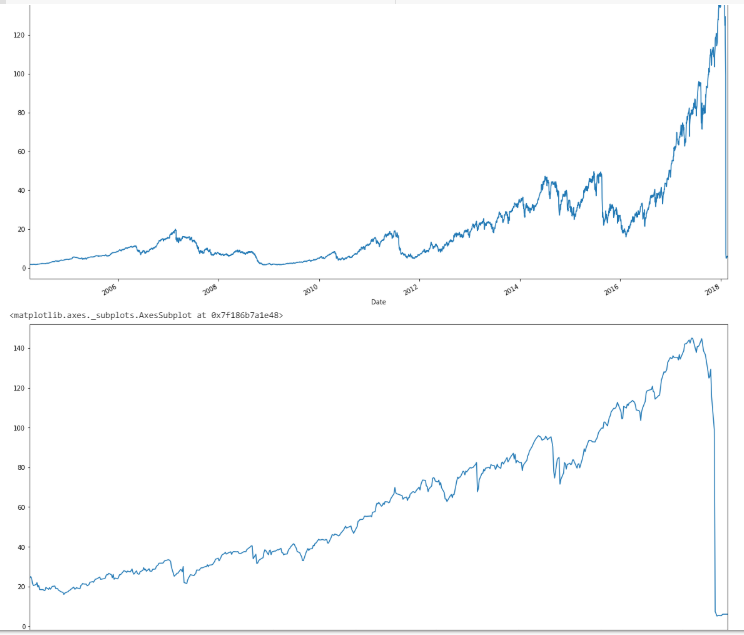
plot(GSPCcumSqRets)

This results in the following image:

So far, so good. Let’s now try to find the amount of changepoints that Dr. Frey’s graph alludes to.

t1 <- Sys.time()
ECPmonthRes <- e.divisive(X = GSPCsqRets, min.size = 2)
t2 <- Sys.time()
print(t2 - t1)

t1 <- Sys.time()
BDmonthRes <- breakout(Z = GSPCsqRets, min.size = 2, beta=0, degree=1)
t2 <- Sys.time()
print(t2 - t1)

ECPmonthRes$estimates
BDres$loc

With the following results:

> ECPmonthRes$estimates
[1]   1 285 293 342
> BDres$loc
[1] 47 87

In short, two changepoints for each. Far from the 20 or so regimes present in Dr. Frey’s analysis. So, not close to anything that was expected. My intuition tells me that the main reason for this is that these algorithms are data-hungry, and there is too little data for them to do much more than what they have done thus far. So let’s go the other way and use daily data.

dailySqRets <- Return.calculate(Cl(GSPC))*Return.calculate(Cl(GSPC))
dailySqRets <- dailySqRets["1985::"]

plot(cumsum(dailySqRets))

And here’s the new plot:

First, let’s try the e-divisive algorithm from the ecp package to find our changepoints, with a minimum size of 20 days between regimes. (Blog note: this is a process that takes an exceptionally long time. For me, it took more than 2 hours.)

t1 <- Sys.time()
ECPres <- e.divisive(X = dailySqRets, min.size=20)
t2 <- Sys.time()
print(t2 - t1)
Time difference of 2.214813 hours

With the following results:

index(dailySqRets)[ECPres$estimates]
 [1] "1985-01-02" "1987-10-14" "1987-11-11" "1998-07-21" "2002-07-01" "2003-07-28" "2008-09-15" "2008-12-09"
 [9] "2009-06-02" NA   

The first and last are merely the endpoints of the data. So essentially, it encapsulates Black Monday and the crisis, among other things. Let’s look at how the algorithm split the volatility regimes. For this, we will use the xtsExtra package for its plotting functionality (thanks to Ross Bennett for the work he did in implementing it).

require(xtsExtra)
plot(cumsum(dailySqRets))
xtsExtra::addLines(index(dailySqRets)[ECPres$estimates[-c(1, length(ECPres$estimates))]], on = 1, col = "blue", lwd = 2)

With the resulting plot:

In this case, the e-divisive algorithm from the ecp package does a pretty great job segmenting the various volatility regimes, as can be thought of roughly as the slope of the cumulative squared returns. The algorithm’s ability to accurately cluster the Black Monday events, along with the financial crisis, shows its industrial-strength applicability. How does this look on the price graph?

plot(Cl(GSPC))
xtsExtra::addLines(index(dailySqRets)[ECPres$estimates[-c(1, length(ECPres$estimates))]], on = 1, col = "blue", lwd = 2)

In this case, Black Monday is clearly visible, along with the end of the Clinton bull run through the dot-com bust, the consolidation, the run-up to the crisis, the crisis itself, the consolidation, and the new bull market.

Note that the presence of a new volatility regime may not necessarily signify a market top or bottom, but the volatility regime detection seems to have worked very well in this case.

For comparison, let’s examine the e-divisive with medians algorithm.

t1 <- Sys.time()
BDres <- breakout(Z = dailySqRets, min.size = 20, beta=0, degree=1)
t2 <- Sys.time()
print(t2-t1)

BDres$loc
index(dailySqRets)[BDres$loc]

With the following result:

Time difference of 2.900167 secs
> BDres$loc
[1] 5978
> BDres$loc
[1] 5978
> index(dailySqRets)[BDres$loc]
[1] "2008-09-12"

So while the algorithm is a lot faster, its volatility regime detection, it only sees the crisis as the one major change point. Beyond that, to my understanding, the e-divisive with medians algorithm may be “too robust” (even without any penalization) against anomalies (after all, the median is robust to changes in 50% of the data). In short, I think that while it clearly has applications, such as twitter cloud production data, it doesn’t seem to obtain a result that’s in the ballpark of two other separate procedures.

Lastly, let’s try and create a plot similar to Dr. Frey’s, with spikes, mountains, and plains.

require(PerformanceAnalytics)
GSPCrets <- Return.calculate(Cl(GSPC))
GSPCrets <- GSPCrets["1985::"]
GSPCrets$regime <- ECPres$cluster
GSPCrets$annVol <- NA

for(i in unique(ECPres$cluster)) {
  regime <- GSPCrets[GSPCrets$regime==i,]
  annVol <- StdDev.annualized(regime[,1])
  GSPCrets$annVol[GSPCrets$regime==i,] <- annVol
}

plot(GSPCrets$annVol, ylim=c(0, max(GSPCrets$annVol)), main="GSPC volatility regimes, 1985 to 2013-05")

With the corresponding image, inspired by Dr. Robert Frey:

This concludes the research replication.

********************************

Whew. Done. While I gained some understanding of what change points are useful for, I won’t profess to be an expert on them (some of the math involved uses PhD-level mathematics such as characteristic functions that I never learned). However, it was definitely interesting pulling together several different ideas and uniting them under a rigorous process.

Special thanks for this blog post:

Brian Peterson, for the process paper and putting a formal structure to the research replication process (and requesting this post).
Robert J. Frey, for the “volatility landscape” idea that I could objectively point to as an objective benchmark to validate the hypothesis of the paper.
David S. Matteson, for the ecp package.
Nicholas A. James, for the work done in the BreakoutDetection package (and clarifying some of its functionality for me).
Arun Kejariwal, for the tutorial on using the BreakoutDetection package.

Thanks for reading.

NOTE: I am a freelance consultant in quantitative analysis on topics related to this blog. If you have contract or full time roles available for proprietary research that could benefit from my skills, please contact me through my LinkedIn here.

Introducing Stepwise Correlation Rank

So in the last post, I attempted to replicate the Flexible Asset Allocation paper. I’d like to offer a thanks to Pat of Intelligent Trading Tech (not updated recently, hopefully this will change) for helping me corroborate the results, so that I have more confidence there isn’t an error in my code.

One of the procedures the authors of the FAA paper used is a correlation rank, which I interpreted as the average correlation of each security to the others.

The issue, pointed out to me in a phone conversation I had with David Varadi is that when considering correlation, shouldn’t the correlations the investor is concerned about be between instruments within the portfolio, as opposed to simply all the correlations, including to instruments not in the portfolio? To that end, when selecting assets (or possibly features in general), conceptually, it makes more sense to select in a stepwise fashion–that is, start off at a subset of the correlation matrix, and then rank assets in order of their correlation to the heretofore selected assets, as opposed to all of them. This was explained in Mr. Varadi’s recent post.

Here’s a work in progress function I wrote to formally code this idea:

stepwiseCorRank <- function(corMatrix, startNames=NULL, stepSize=1, bestHighestRank=FALSE) {
  #edge cases
  if(dim(corMatrix)[1] == 1) {
    return(corMatrix)
  } else if (dim(corMatrix)[1] == 2) {
    ranks <- c(1.5, 1.5)
    names(ranks) <- colnames(corMatrix)
    return(ranks)
  }
  if(is.null(startNames)) {
    corSums <- rowSums(corMatrix)
    corRanks <- rank(corSums)
    startNames <- names(corRanks)[corRanks <= stepSize]
  }
  nameList <- list()
  nameList[[1]] <- startNames
  rankList <- list()
  rankCount <- 1
  rankList[[1]] <- rep(rankCount, length(startNames))
  rankedNames <- do.call(c, nameList)
  
  while(length(rankedNames) < nrow(corMatrix)) {
    rankCount <- rankCount+1
    subsetCor <- corMatrix[, rankedNames]
    if(class(subsetCor) != "numeric") {
      subsetCor <- subsetCor[!rownames(corMatrix) %in% rankedNames,]
      if(class(subsetCor) != "numeric") {
        corSums <- rowSums(subsetCor)
        corSumRank <- rank(corSums)
        lowestCorNames <- names(corSumRank)[corSumRank <= stepSize]
        nameList[[rankCount]] <- lowestCorNames
        rankList[[rankCount]] <- rep(rankCount, min(stepSize, length(lowestCorNames)))
      } else { #1 name remaining
        nameList[[rankCount]] <- rownames(corMatrix)[!rownames(corMatrix) %in% names(subsetCor)]
        rankList[[rankCount]] <- rankCount
      }
    } else {  #first iteration, subset on first name
      subsetCorRank <- rank(subsetCor)
      lowestCorNames <- names(subsetCorRank)[subsetCorRank <= stepSize]
      nameList[[rankCount]] <- lowestCorNames
      rankList[[rankCount]] <- rep(rankCount, min(stepSize, length(lowestCorNames)))
    }    
    rankedNames <- do.call(c, nameList)
  }
  
  ranks <- do.call(c, rankList)
  names(ranks) <- rankedNames
  if(bestHighestRank) {
    ranks <- 1+length(ranks)-ranks
  }
  ranks <- ranks[colnames(corMatrix)] #return to original order
  return(ranks)
}

So the way the function works is that it takes in a correlation matrix, a starting name (if provided), and a step size (that is, how many assets to select per step, so that the process doesn’t become extremely long when dealing with larger amounts of assets/features). Then, it iterates–subset the correlation matrix on the starting name, and find the minimum value, and add it to a list of already-selected names. Next, subset the correlation matrix columns on the selected names, and the rows on the not selected names, and repeat, until all names have been accounted for. Due to R’s little habit of wiping out labels when a matrix becomes a vector, I had to write some special case code, which is the reason for two nested if/else statements (the first one being for the first column subset, and the second being for when there’s only one row remaining).

Also, if there’s an edge case (1 or 2 securities), then there is some functionality to handle those trivial cases.

Here’s a test script I wrote to test this function out:

require(PerformanceAnalytics)
require(quantmod)

#mid 1997 to end of 2012
getSymbols(mutualFunds, from="1997-06-30", to="2012-12-31")
tmp <- list()
for(fund in mutualFunds) {
  tmp[[fund]] <- Ad(get(fund))
}

#always use a list hwne intending to cbind/rbind large quantities of objects
adPrices <- do.call(cbind, args = tmp)
colnames(adPrices) <- gsub(".Adjusted", "", colnames(adPrices))

adRets <- Return.calculate(adPrices)

subset <- adRets["2012"]
corMat <- cor(subset)

tmp <- list()
for(i in 1:length(mutualFunds)) {
  rankRow <- stepwiseCorRank(corMat, startNames=mutualFunds[i])
  tmp[[i]] <- rankRow
}
rankDemo <- do.call(rbind, tmp)
rownames(rankDemo) <- mutualFunds
origRank <- rank(rowSums(corMat))
rankDemo <- rbind(rankDemo, origRank)
rownames(rankDemo)[8] <- "Original (VBMFX)"

heatmap(-rankDemo, Rowv=NA, Colv=NA, col=heat.colors(8), margins=c(6,6))

Essentially, using the 2012 year of returns for the 7 FAA mutual funds, I compared how different starting securities changed the correlation ranking sequence.

Here are the results:

               VTSMX FDIVX VEIEX VFISX VBMFX QRAAX VGSIX
VTSMX              1     6     7     4     2     3     5
FDIVX              6     1     7     4     2     5     3
VEIEX              6     7     1     4     2     3     5
VFISX              2     6     7     1     3     4     5
VBMFX              2     6     7     4     1     3     5
QRAAX              5     6     7     4     2     1     3
VGSIX              5     6     7     4     2     3     1
Non-Sequential     5     6     7     2     1     3     4

In short, the algorithm is rather robust to starting security selection, at least judging by this small example. However, comparing VBMFX start to the non-sequential ranking, we see that VFISX changes from rank 2 in the non-sequential to rank 4, with VTSMX going from rank 5 to rank 2. From an intuitive perspective, this makes sense, as both VBMFX and VFISX are bond funds, which have a low correlation with the other 5 equity-based mutual funds, but a higher correlation with each other, thus signifying that the algorithm seems to be working as intended, at least insofar as this small example demonstrates. Here’s a heatmap to demonstrate this in visual form.

The ranking order (starting security) is the vertical axis, and the horizontal are the ranks, from white being first, to red being last. Notice once again that the ranking orders are robust in general (consider each column of colors descending), but each particular ranking order is unique.

So far, this code still has to be tested in terms of its applications to portfolio management and asset allocation, but for those interested in such an idea, it’s my hope that this provides a good reference point.

Thanks for reading.

Intermission: A Quick Thought on Robust Kurtosis

This post was inspired by some musings from John Bollinger that as data in the financial world wasn’t normally distributed, that there might be a more robust computation to indicate skewness and kurtosis. For instance, one way to think about skewness is the difference between mean and median. That is, if the mean is less than the median, that the distribution was left skewed, and vice versa.

This post attempts to extend that thinking to kurtosis. That is, just as the skew can be thought of as a relationship between mean and median, so too, might kurtosis be thought of as a relationship between two measures of spread–standard deviation and the more robust interquartile range. So, I performed an experiment to simulate 10000 observations from a standard normal and 10000 observations from a standard double-exponential distribution.

Here’s the experiment I ran.

set.seed(1234)
norms <- rnorm(10000)
dexps <- rexp(10000) * sign(rnorm(10000))
plot(density(dexps))
lines(density(norms), col="red")
(IQR(norms))
(IQR(dexps))
(sd(norms))
(sd(dexps))
(sd(norms)/IQR(norms))
(sd(dexps)/IQR(dexps))

And here’s the output:

[1] 0.9757966
> (IQR(norms))
[1] 1.330469
> (IQR(dexps))
[1] 1.35934
> (sd(norms))
[1] 0.9875294
> (sd(dexps))
[1] 1.393057
> (sd(norms)/IQR(norms))
[1] 0.7422415
> (sd(dexps)/IQR(dexps))
[1] 1.024804

That is, in a distribution with higher kurtosis than the standard normal, that the ratio between standard deviation to interquartile range is higher in a heavier-tailed distribution. I’m not certain that this assertion is true in all general cases, but it seems to make intuitive sense, that with heavier tails, the same amount of observations are more spread out.

Thanks for reading.

Comparing ATR order sizing to max dollar order sizing

First off, it has come to my attention that some readers have trouble getting some of my demos to work because there may be different versions of TTR in use. If ever your demo doesn’t work, the first thing I would immediately recommend you do is this:

Only run the code through the add.indicator logic. And then, rather than adding the signals and rules, run the following code:

test <- applyIndicators(strategy.st, mktdata=OHLC(XLB))
head(test)

That should show you the exact column names of your indicators, and you can adjust your inputs accordingly.While one of my first posts introduced the ATR order-sizing function, I recently received a suggestion to test it in the context of whether or not it actually normalized risk across instruments. To keep things simple, my strategy is as plain vanilla as strategies come — RSI2 20/80 filtered on SMA200.

Here’s the code for the ATR order sizing version, for completeness’s sake.

require(IKTrading)
require(quantstrat)
require(PerformanceAnalytics)

initDate="1990-01-01"
from="2003-01-01"
to="2012-12-31"
options(width=70)

source("demoData.R")

#trade sizing and initial equity settings
tradeSize <- 100000
initEq <- tradeSize*length(symbols)

strategy.st <- portfolio.st <- account.st <- "DollarVsATRos"
rm.strat(portfolio.st)
rm.strat(strategy.st)
initPortf(portfolio.st, symbols=symbols, initDate=initDate, currency='USD')
initAcct(account.st, portfolios=portfolio.st, initDate=initDate, currency='USD',initEq=initEq)
initOrders(portfolio.st, initDate=initDate)
strategy(strategy.st, store=TRUE)

#parameters
pctATR=.02
period=10

nRSI <- 2
buyThresh <- 20
sellThresh <- 80
nSMA <- 200

add.indicator(strategy.st, name="lagATR", 
              arguments=list(HLC=quote(HLC(mktdata)), n=period), 
              label="atrX")

add.indicator(strategy.st, name="RSI",
              arguments=list(price=quote(Cl(mktdata)), n=nRSI),
              label="rsi")

add.indicator(strategy.st, name="SMA",
              arguments=list(x=quote(Cl(mktdata)), n=nSMA),
              label="sma")

#signals
add.signal(strategy.st, name="sigComparison",
           arguments=list(columns=c("Close", "sma"), relationship="gt"),
           label="filter")

add.signal(strategy.st, name="sigThreshold",
           arguments=list(column="rsi", threshold=buyThresh, 
                          relationship="lt", cross=FALSE),
           label="rsiLtThresh")

add.signal(strategy.st, name="sigAND",
           arguments=list(columns=c("filter", "rsiLtThresh"), cross=TRUE),
           label="longEntry")

add.signal(strategy.st, name="sigThreshold",
           arguments=list(column="rsi", threshold=sellThresh,
                          relationship="gt", cross=TRUE),
           label="longExit")

add.signal(strategy.st, name="sigCrossover",
           arguments=list(columns=c("Close", "sma"), relationship="lt"),
           label="filterExit")

#rules
add.rule(strategy.st, name="ruleSignal", 
         arguments=list(sigcol="longEntry", sigval=TRUE, ordertype="market", 
                        orderside="long", replace=FALSE, prefer="Open", osFUN=osDollarATR,
                        tradeSize=tradeSize, pctATR=pctATR, atrMod="X"), 
         type="enter", path.dep=TRUE)

add.rule(strategy.st, name="ruleSignal", 
         arguments=list(sigcol="longExit", sigval=TRUE, orderqty="all", ordertype="market", 
                        orderside="long", replace=FALSE, prefer="Open"), 
         type="exit", path.dep=TRUE)

add.rule(strategy.st, name="ruleSignal", 
         arguments=list(sigcol="filterExit", sigval=TRUE, orderqty="all", ordertype="market", 
                        orderside="long", replace=FALSE, prefer="Open"), 
         type="exit", path.dep=TRUE)

#apply strategy
t1 <- Sys.time()
out <- applyStrategy(strategy=strategy.st,portfolios=portfolio.st)
t2 <- Sys.time()
print(t2-t1)

#set up analytics
updatePortf(portfolio.st)
dateRange <- time(getPortfolio(portfolio.st)$summary)[-1]
updateAcct(portfolio.st,dateRange)
updateEndEq(account.st)

Here are some of the usual analytics, which don’t interest me in and of themselves as this strategy is rather throwaway, but to compare them to what happens when I use the max dollar order sizing function in a moment:

> (aggPF <- sum(tStats$Gross.Profits)/-sum(tStats$Gross.Losses))
[1] 1.659305
> (aggCorrect <- mean(tStats$Percent.Positive))
[1] 69.24967
> (numTrades <- sum(tStats$Num.Trades))
[1] 3017
> (meanAvgWLR <- mean(tStats$Avg.WinLoss.Ratio[tStats$Avg.WinLoss.Ratio < Inf], na.rm=TRUE))
[1] 0.733

> SharpeRatio.annualized(portfRets)
                                     [,1]
Annualized Sharpe Ratio (Rf=0%) 0.9783541
> Return.annualized(portfRets)
                        [,1]
Annualized Return 0.07369592
> maxDrawdown(portfRets)
[1] 0.08405041

> round(apply.yearly(dailyRetComparison, Return.cumulative),3)
           strategy    SPY
2003-12-31    0.052  0.066
2004-12-31    0.074  0.079
2005-12-30    0.045  0.025
2006-12-29    0.182  0.132
2007-12-31    0.117  0.019
2008-12-31   -0.010 -0.433
2009-12-31    0.130  0.192
2010-12-31   -0.005  0.110
2011-12-30    0.069 -0.028
2012-12-31    0.087  0.126
> round(apply.yearly(dailyRetComparison, SharpeRatio.annualized),3)
           strategy    SPY
2003-12-31    1.867  3.641
2004-12-31    1.020  0.706
2005-12-30    0.625  0.238
2006-12-29    2.394  1.312
2007-12-31    1.105  0.123
2008-12-31   -0.376 -1.050
2009-12-31    1.752  0.719
2010-12-31   -0.051  0.614
2011-12-30    0.859 -0.122
2012-12-31    1.201  0.990
> round(apply.yearly(dailyRetComparison, maxDrawdown),3)
           strategy   SPY
2003-12-31    0.018 0.025
2004-12-31    0.065 0.085
2005-12-30    0.053 0.074
2006-12-29    0.074 0.077
2007-12-31    0.066 0.102
2008-12-31    0.032 0.520
2009-12-31    0.045 0.280
2010-12-31    0.084 0.167
2011-12-30    0.053 0.207
2012-12-31    0.050 0.099

Now here’s a new bit of analytics–comparing annualized standard deviations between securities:

> sdQuantile <- quantile(sapply(instRets, sd.annualized))
> sdQuantile
         0%         25%         50%         75%        100% 
0.004048235 0.004349390 0.004476377 0.004748530 0.005557765 
> (extremeRatio <- sdQuantile[5]/sdQuantile[1]-1)
    100% 
0.372886 
> (boxBorderRatio <- sdQuantile[4]/sdQuantile[2]-1)
      75% 
0.0917693 

In short, because the instrument returns are computed as a function of only the initial account equity (quantstrat doesn’t know that I’m “allocating” a notional cash amount to each separate ETF–because I’m really not–I just treat it as one pile of cash that I mentally think of as being divided “equally” between all 30 ETFs), that means that the returns per instrument also have already implicitly factored in the weighting scheme from the order sizing function. In this case, the most volatile instrument is about 37% more volatile than the least — and since I’m dealing with indices of small nations along with short-term treasury bills in ETF form, I’d say that’s impressive.

More impressive, in my opinion, is that the difference in volatility between the 25th and 75th percentile is about 9%. It means that our ATR order sizing seems to be doing its job.Here’s the raw computations in terms of annualized volatility:

> sapply(instRets, sd.annualized)
EFA.DailyEndEq EPP.DailyEndEq EWA.DailyEndEq EWC.DailyEndEq 
   0.004787248    0.005557765    0.004897699    0.004305728 
EWG.DailyEndEq EWH.DailyEndEq EWJ.DailyEndEq EWS.DailyEndEq 
   0.004806879    0.004782505    0.004460708    0.004618460 
EWT.DailyEndEq EWU.DailyEndEq EWY.DailyEndEq EWZ.DailyEndEq 
   0.004417686    0.004655716    0.004888876    0.004858743 
EZU.DailyEndEq IEF.DailyEndEq IGE.DailyEndEq IYR.DailyEndEq 
   0.004631333    0.004779468    0.004617250    0.004359273 
IYZ.DailyEndEq LQD.DailyEndEq RWR.DailyEndEq SHY.DailyEndEq 
   0.004346095    0.004101408    0.004388131    0.004585389 
TLT.DailyEndEq XLB.DailyEndEq XLE.DailyEndEq XLF.DailyEndEq 
   0.004392335    0.004319708    0.004515228    0.004426415 
XLI.DailyEndEq XLK.DailyEndEq XLP.DailyEndEq XLU.DailyEndEq 
   0.004129331    0.004492046    0.004369804    0.004048235 
XLV.DailyEndEq XLY.DailyEndEq 
   0.004148445    0.004203503 

And here’s a histogram of those same calculations:

In this case, the reason that the extreme computation gives us a 37% greater result is that one security, EPP (pacific ex-Japan, which for all intents and purposes is emerging markets) is simply out there a bit. The rest just seem very clumped up.

Now let’s remove the ATR order sizing and replace it with a simple osMaxDollar rule, that simply will keep a position topped off at a notional dollar value. In short, aside from a few possible one-way position rebalancing transactions (E.G. with the ATR order sizing rule, ATR may have gone up whereas total value of a position may have gone down, which may trigger the osMaxDollar rule but not the osDollarATR rule on a second RSI cross) Here’s the new entry rule, with the ATR commented out:

# add.rule(strategy.st, name="ruleSignal", 
#          arguments=list(sigcol="longEntry", sigval=TRUE, ordertype="market", 
#                         orderside="long", replace=FALSE, prefer="Open", osFUN=osDollarATR,
#                         tradeSize=tradeSize, pctATR=pctATR, atrMod="X"), 
#          type="enter", path.dep=TRUE)

add.rule(strategy.st, name="ruleSignal", 
         arguments=list(sigcol="longEntry", sigval=TRUE, ordertype="market", 
                        orderside="long", replace=FALSE, prefer="Open", osFUN=osMaxDollar,
                        tradeSize=tradeSize, maxSize=tradeSize), 
         type="enter", path.dep=TRUE)

Let’s look at the corresponding statistical results:

> (aggPF <- sum(tStats$Gross.Profits)/-sum(tStats$Gross.Losses))
[1] 1.635629
> (aggCorrect <- mean(tStats$Percent.Positive))
[1] 69.45633
> (numTrades <- sum(tStats$Num.Trades))
[1] 3019
> (meanAvgWLR <- mean(tStats$Avg.WinLoss.Ratio[tStats$Avg.WinLoss.Ratio < Inf], na.rm=TRUE))
[1] 0.735

> SharpeRatio.annualized(portfRets)
                                     [,1]
Annualized Sharpe Ratio (Rf=0%) 0.8529713
> Return.annualized(portfRets)
                        [,1]
Annualized Return 0.04857159
> maxDrawdown(portfRets)
[1] 0.06682969
> 
> dailyRetComparison <- cbind(portfRets, SPYrets)
> colnames(dailyRetComparison)  <- c("strategy", "SPY")
> round(apply.yearly(dailyRetComparison, Return.cumulative),3)
           strategy    SPY
2003-12-31    0.034  0.066
2004-12-31    0.055  0.079
2005-12-30    0.047  0.025
2006-12-29    0.090  0.132
2007-12-31    0.065  0.019
2008-12-31   -0.023 -0.433
2009-12-31    0.141  0.192
2010-12-31   -0.010  0.110
2011-12-30    0.038 -0.028
2012-12-31    0.052  0.126
> round(apply.yearly(dailyRetComparison, SharpeRatio.annualized),3)
           strategy    SPY
2003-12-31    1.639  3.641
2004-12-31    1.116  0.706
2005-12-30    0.985  0.238
2006-12-29    1.755  1.312
2007-12-31    0.785  0.123
2008-12-31   -0.856 -1.050
2009-12-31    1.774  0.719
2010-12-31   -0.134  0.614
2011-12-30    0.686 -0.122
2012-12-31    1.182  0.990
> round(apply.yearly(dailyRetComparison, maxDrawdown),3)
           strategy   SPY
2003-12-31    0.015 0.025
2004-12-31    0.035 0.085
2005-12-30    0.033 0.074
2006-12-29    0.058 0.077
2007-12-31    0.058 0.102
2008-12-31    0.036 0.520
2009-12-31    0.043 0.280
2010-12-31    0.062 0.167
2011-12-30    0.038 0.207
2012-12-31    0.035 0.099

And now for the kicker–to see just how much riskier using a naive order-sizing method that doesn’t take into account the different idiosyncratic of a security is:

> sdQuantile <- quantile(sapply(instRets, sd.annualized))
> sdQuantile
          0%          25%          50%          75%         100% 
0.0002952884 0.0026934043 0.0032690492 0.0037727970 0.0061480828 
> (extremeRatio <- sdQuantile[5]/sdQuantile[1]-1)
   100% 
19.8206 
> (boxBorderRatio <- sdQuantile[4]/sdQuantile[2]-1)
     75% 
0.400754 
> hist(sapply(instRets, sd.annualized))

In short, the ratio between the riskiest and least riskiest asset rises from less than 40% to 1900%. But in case, that’s too much of an outlier (E.G. dealing with treasury bill/note/bond ETFs vs. pacific ex-Japan aka emerging Asia), the difference between the third and first quartiles in terms of volatility ratio has jumped from 9% to 40%.

Here’s the corresponding histogram:
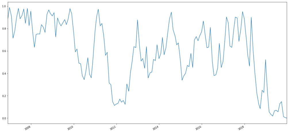
As can be seen, a visibly higher variance in variances–in other words, a second moment on the second moment–meaning that to not use an order-sizing function that takes into account individual security risk therefore introduces unnecessary kurtosis and heavier tails into the risk/reward ratio, and due to this unnecessary excess risk, performance suffers measurably.Here are the individual security annualized standard deviations for the max dollar order sizing method:

> sapply(instRets, sd.annualized)
EFA.DailyEndEq EPP.DailyEndEq EWA.DailyEndEq EWC.DailyEndEq 
  0.0029895232   0.0037767697   0.0040222015   0.0036137500 
EWG.DailyEndEq EWH.DailyEndEq EWJ.DailyEndEq EWS.DailyEndEq 
  0.0037097070   0.0039615376   0.0030398638   0.0037608791 
EWT.DailyEndEq EWU.DailyEndEq EWY.DailyEndEq EWZ.DailyEndEq 
  0.0041140227   0.0032204771   0.0047719772   0.0061480828 
EZU.DailyEndEq IEF.DailyEndEq IGE.DailyEndEq IYR.DailyEndEq 
  0.0033176214   0.0013059712   0.0041621776   0.0033752435 
IYZ.DailyEndEq LQD.DailyEndEq RWR.DailyEndEq SHY.DailyEndEq 
  0.0026899679   0.0011777797   0.0034789117   0.0002952884 
TLT.DailyEndEq XLB.DailyEndEq XLE.DailyEndEq XLF.DailyEndEq 
  0.0024854557   0.0034895815   0.0043568967   0.0029546665 
XLI.DailyEndEq XLK.DailyEndEq XLP.DailyEndEq XLU.DailyEndEq 
  0.0027963302   0.0028882028   0.0021212224   0.0025802850 
XLV.DailyEndEq XLY.DailyEndEq 
  0.0020399289   0.0027037138

Is ATR order sizing the absolute best order-sizing methodology? Most certainly not.In fact, in the PortfolioAnalytics package (quantstrat’s syntax was modeled from this), there are ways to explicitly penalize the higher order moments and co-moments. However, in this case, ATR order sizing works as a simple yet somewhat effective demonstrator of risk-adjusted order-sizing, while implicitly combating some of the risks in not paying attention to the higher moments of the distributions of returns, and also still remaining fairly close to the shore in terms of ease of explanation to those without heavy quantitative backgrounds. This facilitates marketing to large asset managers that may otherwise be hesitant in investing with a more complex strategy that they may not so easily understand.

Thanks for reading.